INTERACT Saskatoon Participant VERITAS Summary - W1
Benoit THIERRY
04 April, 2024
1 VERITAS dataset description
Unlike the Eligibility or Health questionnaires, which can mostly be encoded as a flat table, the VERITAS questionnaire implicitly records a series of entities and their relationships:
- Places: list of geocoded locations visited by participants, along with the following characteristics: category, name, visit frequency, transportation mode
- Social contacts: people and/or groups frequented by participants
- Relationships: between social contacts (who knows who / who belongs to which group) as well as between locations and social contacts (places visited along with whom)
The diagram below illustrates the various entities collected throught the VERITAS questionnaire:
2 Basic descriptive statistics
2.1 Section 1: Residence and Neighbourhood
2.1.1 Now, let’s start with your home. What is your address?
home_location <- locations[locations$location_category == 1, ]

## version ggmap
skt_aoi <- st_bbox(filter(home_location, interact_id != "302386742"))
names(skt_aoi) <- c("left", "bottom", "right", "top")
skt_aoi[["left"]] <- skt_aoi[["left"]] - .05
skt_aoi[["right"]] <- skt_aoi[["right"]] + .05
skt_aoi[["top"]] <- skt_aoi[["top"]] + .01
skt_aoi[["bottom"]] <- skt_aoi[["bottom"]] - .01

bm <- get_stadiamap(skt_aoi, zoom = 11, maptype = "stamen_toner_lite") %>%
  ggmap(extent = "device")
bm + geom_sf(data = st_jitter(home_location, .008), inherit.aes = FALSE, color = "blue", size = 1.8, alpha = .3) # see https://github.com/r-spatial/sf/issues/336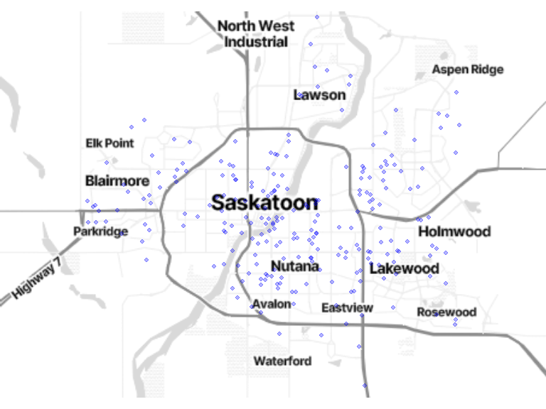
NB: Home locations have been randomly shifted from their original position to protect privacy.
# Number of participants by municipalites
home_by_municipalites <- st_join(home_location, municipalities["NAME"])
home_by_mun_cnt <- home_by_municipalites %>%
  as.data.frame() %>%
  group_by(NAME) %>%
  dplyr::count() %>%
  arrange(desc(n), NAME)
home_by_mun_cnt$geom <- NULL
kable(home_by_mun_cnt, caption = "Number of participants by municipalities") %>% kable_styling(bootstrap_options = "striped", full_width = T, position = "left")| NAME | n |
|---|---|
| Saskatoon | 238 |
| Leask No. 464 | 1 |
2.1.2 When did you move to your current address?
# N of addresses by date of move
year_of_move <- veritas_main[c("interact_id", "home_move_date")]
year_of_move$home_move_date <- year(ymd(year_of_move$home_move_date))
ggplot(data = year_of_move) +
  geom_histogram(aes(x = home_move_date))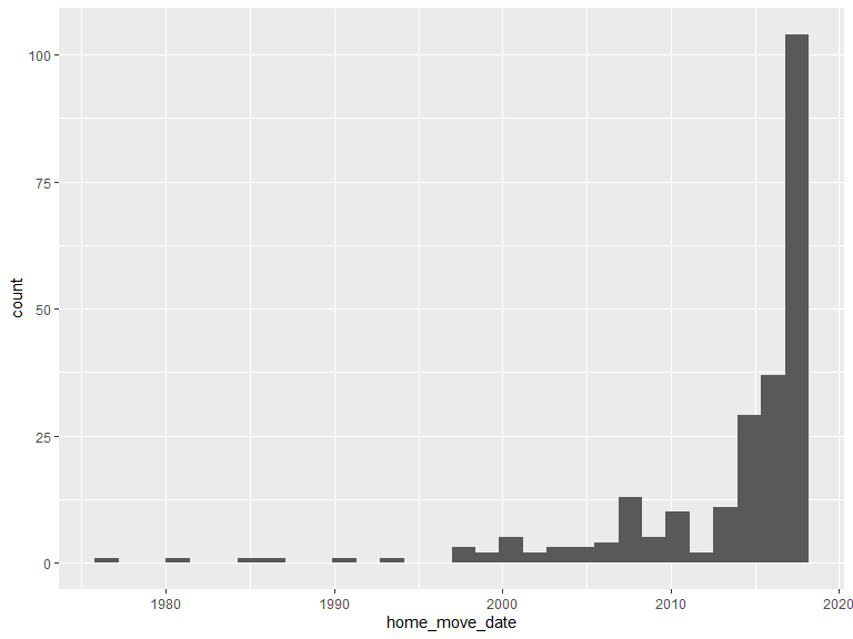
# recode date of move
year_of_move$home_move_date_recode <- as.character(year_of_move$home_move_date)
year_of_move$home_move_date_recode[year_of_move$home_move_date <= 2005] <- "2005 - 2001"
year_of_move$home_move_date_recode[year_of_move$home_move_date <= 2000] <- "2000 - 1991"
year_of_move$home_move_date_recode[year_of_move$home_move_date <= 1990] <- paste("1990 -", min(year_of_move$home_move_date))

year_of_move_cnt <- year_of_move %>%
  group_by(home_move_date_recode) %>%
  dplyr::count() %>%
  arrange(desc(home_move_date_recode))
kable(year_of_move_cnt, caption = "Year of move to current address") %>% kable_styling(bootstrap_options = "striped", full_width = T, position = "left")| home_move_date_recode | n |
|---|---|
| 2018 | 72 |
| 2017 | 32 |
| 2016 | 37 |
| 2015 | 15 |
| 2014 | 14 |
| 2013 | 11 |
| 2012 | 2 |
| 2011 | 5 |
| 2010 | 5 |
| 2009 | 5 |
| 2008 | 8 |
| 2007 | 5 |
| 2006 | 4 |
| 2005 - 2001 | 10 |
| 2000 - 1991 | 10 |
| 1990 - 1977 | 4 |
2.1.3 If you were asked to draw the boundaries of your neighbourhood, what would they be?
prn <- poly_geom[poly_geom$area_type == "neighborhood", ]

## version ggmap
bm + geom_sf(data = prn, inherit.aes = FALSE, fill = alpha("blue", 0.05), color = alpha("blue", 0.3))
# Min, max, median & mean area of PRN
prn$area_m2 <- st_area(prn$geom)
kable(t(as.matrix(summary(prn$area_m2))),
  caption = "Area (in square meters) of the perceived residential neighborhood",
  digits = 1
) %>%
kable_styling(bootstrap_options = "striped", full_width = T, position = "left")| Min. | 1st Qu. | Median | Mean | 3rd Qu. | Max. |
|---|---|---|---|---|---|
| 43.7 | 247186.2 | 865574.3 | 1115337 | 1586445 | 10110206 |
NB only 199 valid neighborhoods were collected, as many participants struggled to draw polygons on the map.
2.1.4 How attached are you to your neighbourhood?
# extract and recode
.ngh_att <- veritas_main[veritas_main$neighbourhood_attach != 99, c("interact_id", "neighbourhood_attach")] %>% dplyr::rename(neighbourhood_attach_code = neighbourhood_attach)
.ngh_att$neighbourhood_attach <- factor(ifelse(.ngh_att$neighbourhood_attach_code == 1, "1 [Not attached at all]",
  ifelse(.ngh_att$neighbourhood_attach_code == 6, "6 [Very attached]",
    .ngh_att$neighbourhood_attach_code
  )
))

# histogram of attachment
ggplot(data = .ngh_att) +
  geom_histogram(aes(x = neighbourhood_attach), stat = "count") +
  scale_x_discrete(labels = function(lbl) str_wrap(lbl, width = 20)) +
  labs(x = "neighbourhood_attach")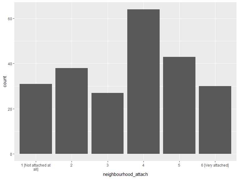
.ngh_att_cnt <- .ngh_att %>%
  group_by(neighbourhood_attach) %>%
  dplyr::count() %>%
  arrange(neighbourhood_attach)
kable(.ngh_att_cnt, caption = "Neigbourhood attachment") %>%
kable_styling(bootstrap_options = "striped", full_width = T, position = "left")| neighbourhood_attach | n |
|---|---|
| 1 [Not attached at all] | 31 |
| 2 | 38 |
| 3 | 27 |
| 4 | 64 |
| 5 | 43 |
| 6 [Very attached] | 30 |
2.1.5 On average, how many hours per day do you spend outside of your home?
# histogram of n hours out
ggplot(data = veritas_main) +
  geom_histogram(aes(x = hours_out))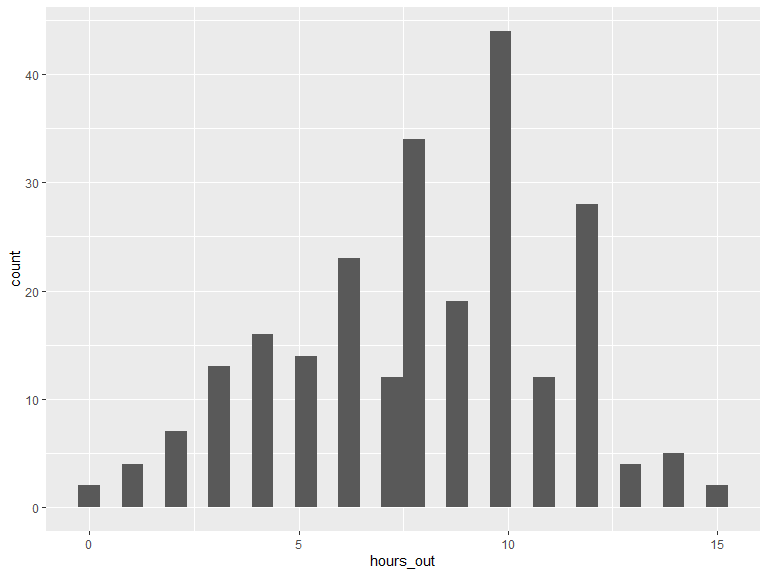
# Min, max, median & mean hours/day out
kable(t(as.matrix(summary(veritas_main$hours_out))),
  caption = "Hours/day outside home",
  digits = 1
) %>%
kable_styling(bootstrap_options = "striped", full_width = T, position = "left")| Min. | 1st Qu. | Median | Mean | 3rd Qu. | Max. |
|---|---|---|---|---|---|
| 0 | 6 | 8 | 8 | 10 | 15 |
2.1.6 Of this time spent outside your home, on average how many hours do you spend outside your neighbourhood?
# histogram of n hours out
ggplot(data = veritas_main) +
  geom_histogram(aes(x = hours_out_neighb))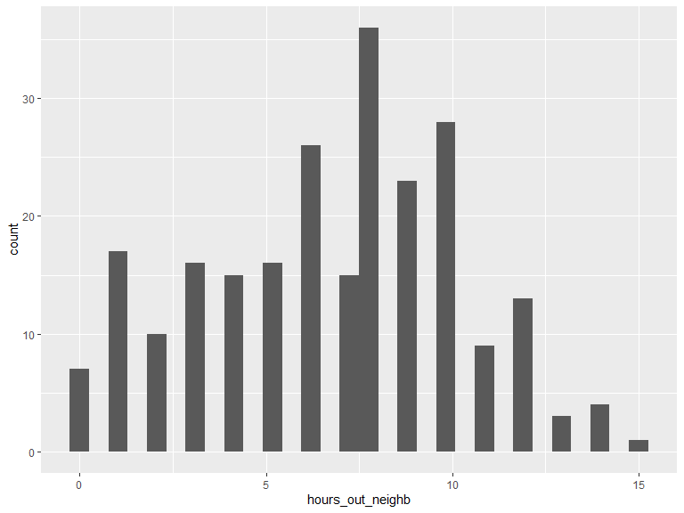
# Min, max, median & mean hours/day out of neighborhood
kable(t(as.matrix(summary(veritas_main$hours_out_neighb))),
  caption = "Hours/day outside neighbourhood",
  digits = 1
) %>%
kable_styling(bootstrap_options = "striped", full_width = T, position = "left")| Min. | 1st Qu. | Median | Mean | 3rd Qu. | Max. |
|---|---|---|---|---|---|
| 0 | 4 | 7 | 6.8 | 9 | 15 |
2.1.7 Are there one or more areas close to where you live that you tend to avoid because you do not feel safe there (for any reason)?
# extract and recode
.unsafe <- veritas_main[c("interact_id", "unsafe_area")] %>% dplyr::rename(unsafe_area_code = unsafe_area)
.unsafe$unsafe_area <- factor(ifelse(.unsafe$unsafe_area_code == 1, "1 [Yes]",
  ifelse(.unsafe$unsafe_area_code == 2, "2 [No]", "N/A")
))

# histogram of answers
ggplot(data = .unsafe) +
  geom_histogram(aes(x = unsafe_area), stat = "count") +
  scale_x_discrete(labels = function(lbl) str_wrap(lbl, width = 20)) +
  labs(x = "unsafe_area")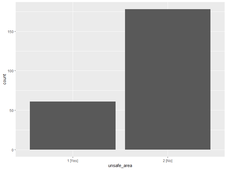
.unsafe_cnt <- .unsafe %>%
  group_by(unsafe_area) %>%
  dplyr::count() %>%
  arrange(unsafe_area)
kable(.unsafe_cnt, caption = "unsafe_area") %>% kable_styling(bootstrap_options = "striped", full_width = T, position = "left")| unsafe_area | n |
|---|---|
| 1 [Yes] | 61 |
| 2 [No] | 178 |
# map
unsafe <- poly_geom[poly_geom$area_type == "unsafe area", ]

## version ggmap
bm + geom_sf(data = unsafe, inherit.aes = FALSE, fill = alpha("blue", 0.3), color = alpha("blue", 0.5))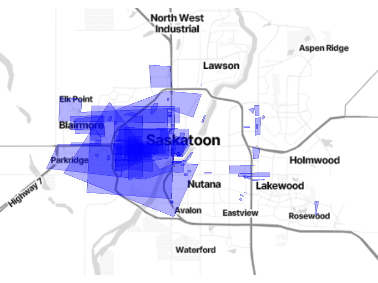
# Min, max, median & mean area of PRN
unsafe$area_m2 <- st_area(unsafe$geom)
kable(t(as.matrix(summary(unsafe$area_m2))),
  caption = "Area (in square meters) of the perceived unsafe area",
  digits = 1
) %>%
kable_styling(bootstrap_options = "striped", full_width = T, position = "left")| Min. | 1st Qu. | Median | Mean | 3rd Qu. | Max. |
|---|---|---|---|---|---|
| 110.6 | 22383 | 121791 | 1839207 | 757198.2 | 23790304 |
2.1.8 Do you spend the night somewhere other than your home at least once per week?
# extract and recode
.o_res <- veritas_main[c("interact_id", "other_resid")] %>% dplyr::rename(other_resid_code = other_resid)
.o_res$other_resid <- factor(ifelse(.o_res$other_resid_code == 1, "1 [Yes]",
  ifelse(.o_res$other_resid_code == 2, "2 [No]", "N/A")
))

# histogram of answers
ggplot(data = .o_res) +
  geom_histogram(aes(x = other_resid), stat = "count") +
  scale_x_discrete(labels = function(lbl) str_wrap(lbl, width = 20)) +
  labs(x = "other_resid")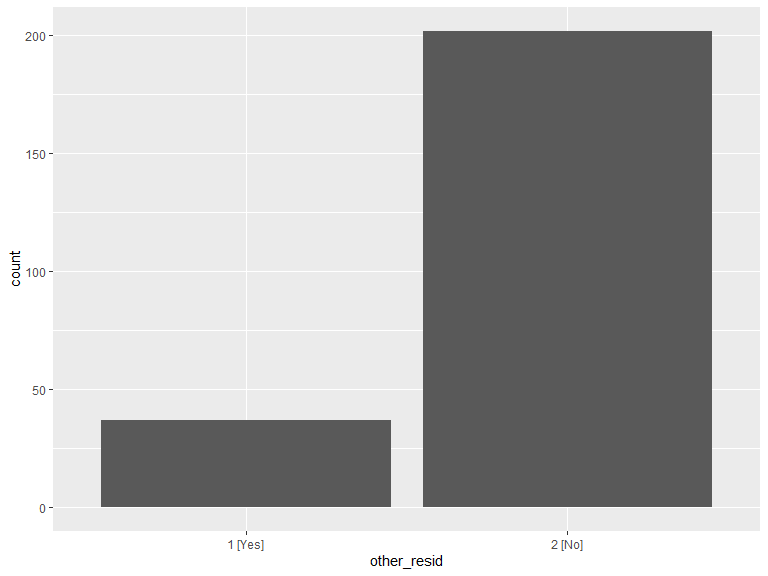
.o_res_cnt <- .o_res %>%
  group_by(other_resid) %>%
  dplyr::count() %>%
  arrange(other_resid)
kable(.o_res_cnt, caption = "Other residence") %>%
kable_styling(bootstrap_options = "striped", full_width = T, position = "left")| other_resid | n |
|---|---|
| 1 [Yes] | 37 |
| 2 [No] | 202 |
2.2 Section 2: Occupation
2.2.1 Are you currently working?
# extract and recode
.work <- veritas_main[c("interact_id", "working")] %>% dplyr::rename(working_code = working)
.work$working <- factor(ifelse(.work$working_code == 1, "1 [Yes]",
  ifelse(.work$working_code == 2, "2 [No]", "N/A")
))

# histogram of answers
ggplot(data = .work) +
  geom_histogram(aes(x = working), stat = "count") +
  scale_x_discrete(labels = function(lbl) str_wrap(lbl, width = 20)) +
  labs(x = "working")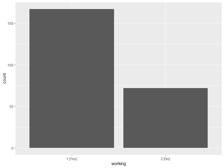
.work_cnt <- .work %>%
  group_by(working) %>%
  dplyr::count() %>%
  arrange(working)
kable(.work_cnt, caption = "Currently working") %>%
kable_styling(bootstrap_options = "striped", full_width = T, position = "left")| working | n |
|---|---|
| 1 [Yes] | 167 |
| 2 [No] | 72 |
2.2.2 Where do you work?
work_location <- locations[locations$location_category == 3, ]

bm + geom_sf(data = work_location, inherit.aes = FALSE, color = "blue", size = 1.8, alpha = .3)
2.2.3 On average, how many hours per week do you work?
# histogram of n hours out
ggplot(data = veritas_main[veritas_main$working == 1, ]) +
  geom_histogram(aes(x = work_hours))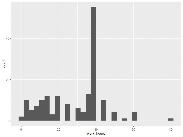
# Min, max, median & mean hours/day out
kable(t(as.matrix(summary(veritas_main$work_hours[veritas_main$working == 1]))),
  caption = "Work hours/week",
  digits = 1
) %>%
kable_styling(bootstrap_options = "striped", full_width = T, position = "left")| Min. | 1st Qu. | Median | Mean | 3rd Qu. | Max. |
|---|---|---|---|---|---|
| 0 | 15 | 35 | 29 | 40 | 80 |
2.2.4 Which of the following categories best describes the amount of physical activity required for your job?
# extract and recode
.work_pa <- veritas_main[veritas_main$working == 1, c("interact_id", "work_pa")] %>% dplyr::rename(work_pa_code = work_pa)
.work_pa$work_pa <- factor(ifelse(.work_pa$work_pa_code == 1, "1 [Mainly sitting with slight arm movements]",
  ifelse(.work_pa$work_pa_code == 2, "2 [Sitting and standing with some walking]",
    ifelse(.work_pa$work_pa_code == 3, "3 [Walking, with some handling of materials generally weighing less than 25 kg (55 lbs)]",
      ifelse(.work_pa$work_pa_code == 4, "4 [Walking and heavy manual work often requiring handling of materials weighing over 25 kg (50 lbs)]", "N/A")
    )
  )
))

# histogram of answers
ggplot(data = .work_pa) +
  geom_histogram(aes(x = work_pa), stat = "count") +
  scale_x_discrete(labels = function(lbl) str_wrap(lbl, width = 20)) +
  labs(x = "Physical activity at work")
.work_pa_cnt <- .work_pa %>%
  group_by(work_pa) %>%
  dplyr::count() %>%
  arrange(work_pa)
kable(.work_pa_cnt, caption = "Physical activity at work") %>% kable_styling(bootstrap_options = "striped", full_width = T, position = "left")| work_pa | n |
|---|---|
| 1 [Mainly sitting with slight arm movements] | 45 |
| 2 [Sitting and standing with some walking] | 57 |
| 3 [Walking, with some handling of materials generally weighing less than 25 kg (55 lbs)] | 60 |
| 4 [Walking and heavy manual work often requiring handling of materials weighing over 25 kg (50 lbs)] | 5 |
2.2.5 Are you currently a registered student?
# extract and recode
.study <- veritas_main[c("interact_id", "studying")] %>% dplyr::rename(studying_code = studying)
.study$studying <- factor(ifelse(.study$studying_code == 1, "1 [Yes]",
  ifelse(.study$studying_code == 2, "2 [No]", "N/A")
))

# histogram of answers
ggplot(data = .study) +
  geom_histogram(aes(x = studying), stat = "count") +
  scale_x_discrete(labels = function(lbl) str_wrap(lbl, width = 20)) +
  labs(x = "Studying")
.study_cnt <- .study %>%
  group_by(studying) %>%
  dplyr::count() %>%
  arrange(studying)
kable(.study_cnt, caption = "Currently studying") %>% kable_styling(bootstrap_options = "striped", full_width = T, position = "left")| studying | n |
|---|---|
| 1 [Yes] | 114 |
| 2 [No] | 125 |
2.2.6 Where do you study?
study_location <- locations[locations$location_category == 4, ]

bm + geom_sf(data = study_location, inherit.aes = FALSE, color = "blue", size = 1.8, alpha = .3)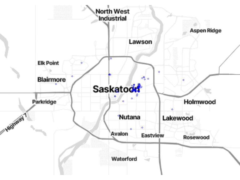
2.2.7 On average, how many hours per week do you study?
# histogram of n hours out
ggplot(data = veritas_main[veritas_main$studying == 1, ]) +
  geom_histogram(aes(x = study_hours))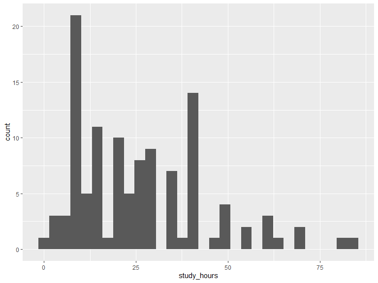
# Min, max, median & mean hours/day out
kable(t(as.matrix(summary(veritas_main$study_hours[veritas_main$studying == 1]))),
  caption = "study hours/week",
  digits = 1
) %>%
kable_styling(bootstrap_options = "striped", full_width = T, position = "left")| Min. | 1st Qu. | Median | Mean | 3rd Qu. | Max. |
|---|---|---|---|---|---|
| 0 | 12 | 23 | 26.2 | 39.2 | 84 |
2.3 Section 3: Shopping activities
The following questions are used to generate the locations grouped into this section:
- Do you shop for groceries at a supermarket at least once per month?
- Do you shop at a public/farmer’s market at least once per month?
- Do you shop at a bakery at least once per month?
- Do you go to a specialty food store at least once per month? For example: a cheese shop, fruit and vegetable store, butcher’s shop, natural and health food store.
- Do you go to a convenience store at least once per month?
- Do you go to a liquor store at least once per month?
shop_location <- locations[locations$location_category %in% c(5, 6, 7, 8, 9, 10), ] %>% dplyr::rename(location_category_code = location_category)
shop_location$location_category <- factor(ifelse(shop_location$location_category_code == 5, " 5 [Supermarket]",
  ifelse(shop_location$location_category_code == 6, " 6 [Public/farmer’s market]",
    ifelse(shop_location$location_category_code == 7, " 7 [Bakery]",
      ifelse(shop_location$location_category_code == 8, " 8 [Specialty food store]",
        ifelse(shop_location$location_category_code == 9, " 9 [Convenience store/Dépanneur]", "10 [Liquor store/SAQ]")
      )
    )
  )
))

# map
bm + geom_sf(data = shop_location, inherit.aes = FALSE, aes(color = location_category), size = 1.5, alpha = .3) +
  scale_color_brewer(palette = "Accent") +
  theme(legend.position = "bottom", legend.text = element_text(size = 8), legend.title = element_blank())
# compute number of shopping locations by category
ggplot(data = shop_location) +
  geom_histogram(aes(x = location_category), stat = "count") +
  scale_x_discrete(labels = function(lbl) str_wrap(lbl, width = 20)) +
  labs(x = "Shopping locations by categories")
.location_category_cnt <- as.data.frame(shop_location[c("location_category")]) %>%
  group_by(location_category) %>%
  dplyr::count() %>%
  arrange(location_category)
kable(.location_category_cnt, caption = "Shopping locations by categories") %>% kable_styling(bootstrap_options = "striped", full_width = T, position = "left")| location_category | n |
|---|---|
| 5 [Supermarket] | 558 |
| 6 [Public/farmer’s market] | 59 |
| 7 [Bakery] | 48 |
| 8 [Specialty food store] | 82 |
| 9 [Convenience store/Dépanneur] | 153 |
| 10 [Liquor store/SAQ] | 137 |
# compute statistics on shopping locations by participants and categories
# > one needs to account for participants who did not report location for some categories
.loc_iid_category_cnt <- as.data.frame(shop_location[c("interact_id", "location_category")]) %>%
  group_by(interact_id, location_category) %>%
  dplyr::count()

# (cont'd) simulate SQL JOIN TABLE ON TRUE
.dummy <- data.frame(
  interact_iid = character(),
  location_category = character()
)
for (iid in as.vector(veritas_main$interact_id)) {
  .dmy <- distinct(.loc_iid_category_cnt[c("location_category")])
  .dmy$interact_id <- as.character(iid)
  .dummy <- rbind(.dummy, .dmy)
}

# (cont'd) find iid/categ combination without match in veritas locations
.no_shop_iid <- dplyr::setdiff(.dummy, .loc_iid_category_cnt[c("location_category", "interact_id")]) %>%
  mutate(n = 0)
.loc_iid_category_cnt <- bind_rows(.loc_iid_category_cnt, .no_shop_iid)

.location_category_cnt <- .loc_iid_category_cnt %>%
  group_by(location_category) %>%
  dplyr::summarise(min = min(n), mean = round(mean(n), 2), median = median(n), max = max(n)) %>%
  arrange(location_category)
kable(.location_category_cnt, caption = "Number of shopping locations by participant and category") %>% kable_styling(bootstrap_options = "striped", full_width = T, position = "left")| location_category | min | mean | median | max |
|---|---|---|---|---|
| 5 [Supermarket] | 0 | 2.33 | 2 | 5 |
| 6 [Public/farmer’s market] | 0 | 0.25 | 0 | 3 |
| 7 [Bakery] | 0 | 0.20 | 0 | 5 |
| 8 [Specialty food store] | 0 | 0.34 | 0 | 4 |
| 9 [Convenience store/Dépanneur] | 0 | 0.64 | 0 | 5 |
| 10 [Liquor store/SAQ] | 0 | 0.57 | 0 | 5 |
2.4 Section 4: Services
The following questions are used to generate the locations grouped into this section:
- Where is the bank you go to most often located?
- Where is the hair salon or barber shop you go to most often?
- Where is the post office where you go to most often?
- Where is the drugstore you go to most often?
- If you need to visit a doctor or other healthcare provider, where do you go most often?
serv_location <- locations[locations$location_category %in% c(11, 12, 13, 14, 15), ] %>% dplyr::rename(location_category_code = location_category)
serv_location$location_category <- factor(ifelse(serv_location$location_category_code == 11, "11 [Bank]",
  ifelse(serv_location$location_category_code == 12, "12 [Hair salon/barbershop]",
    ifelse(serv_location$location_category_code == 13, "13 [Post office]",
      ifelse(serv_location$location_category_code == 14, "14 [Drugstore]", "15 Doctor/healthcare provider]")
    )
  )
))

# map
bm + geom_sf(data = serv_location, inherit.aes = FALSE, aes(color = location_category), size = 1.5, alpha = .3) +
  scale_color_brewer(palette = "Accent") +
  theme(legend.position = "bottom", legend.text = element_text(size = 8), legend.title = element_blank())
# compute number of shopping locations by category
ggplot(data = serv_location) +
  geom_histogram(aes(x = location_category), stat = "count") +
  scale_x_discrete(labels = function(lbl) str_wrap(lbl, width = 20)) +
  labs(x = "Shopping locations by categories")
.location_category_cnt <- as.data.frame(serv_location[c("location_category")]) %>%
  group_by(location_category) %>%
  dplyr::count() %>%
  arrange(location_category)
kable(.location_category_cnt, caption = "Shopping locations by categories") %>% kable_styling(bootstrap_options = "striped", full_width = T, position = "left")| location_category | n |
|---|---|
| 11 [Bank] | 124 |
| 12 [Hair salon/barbershop] | 96 |
| 13 [Post office] | 91 |
| 14 [Drugstore] | 148 |
| 15 Doctor/healthcare provider] | 195 |
# compute statistics on shopping locations by participants and categories
# > one needs to account for participants who did not report location for some categories
.loc_iid_category_cnt <- as.data.frame(serv_location[c("interact_id", "location_category")]) %>%
  group_by(interact_id, location_category) %>%
  dplyr::count()

# (cont'd) simulate SQL JOIN TABLE ON TRUE
.dummy <- data.frame(
  interact_iid = character(),
  location_category = character()
)
for (iid in as.vector(veritas_main$interact_id)) {
  .dmy <- distinct(.loc_iid_category_cnt[c("location_category")])
  .dmy$interact_id <- as.character(iid)
  .dummy <- rbind(.dummy, .dmy)
}

# (cont'd) find iid/categ combination without match in veritas locations
.no_serv_iid <- dplyr::setdiff(.dummy, .loc_iid_category_cnt[c("location_category", "interact_id")]) %>%
  mutate(n = 0)
.loc_iid_category_cnt <- bind_rows(.loc_iid_category_cnt, .no_serv_iid)

.location_category_cnt <- .loc_iid_category_cnt %>%
  group_by(location_category) %>%
  dplyr::summarise(min = min(n), mean = round(mean(n), 2), median = median(n), max = max(n)) %>%
  arrange(location_category)
kable(.location_category_cnt, caption = "Number of shopping locations by participant and category") %>% kable_styling(bootstrap_options = "striped", full_width = T, position = "left")| location_category | min | mean | median | max |
|---|---|---|---|---|
| 11 [Bank] | 0 | 0.52 | 1 | 1 |
| 12 [Hair salon/barbershop] | 0 | 0.40 | 0 | 1 |
| 13 [Post office] | 0 | 0.38 | 0 | 1 |
| 14 [Drugstore] | 0 | 0.62 | 1 | 1 |
| 15 Doctor/healthcare provider] | 0 | 0.82 | 1 | 4 |
2.5 Section 5: Transportation
2.5.1 Do you use public transit from your home?
# extract and recode
.transp <- veritas_main[c("interact_id", "public_transit")] %>% dplyr::rename(public_transit_code = public_transit)
.transp$public_transit <- factor(ifelse(.transp$public_transit_code == 1, "1 [Yes]",
  ifelse(.transp$public_transit_code == 2, "2 [No]", "N/A")
))

# histogram of answers
ggplot(data = .transp) +
  geom_histogram(aes(x = public_transit), stat = "count") +
  scale_x_discrete(labels = function(lbl) str_wrap(lbl, width = 20)) +
  labs(x = "public_transit")
.transp_cnt <- .transp %>%
  group_by(public_transit) %>%
  dplyr::count() %>%
  arrange(public_transit)
kable(.transp_cnt, caption = "Use public transit") %>% kable_styling(bootstrap_options = "striped", full_width = T, position = "left")| public_transit | n |
|---|---|
| 1 [Yes] | 213 |
| 2 [No] | 26 |
2.5.2 Where are the public transit stops that you access from your home?
transp_location <- locations[locations$location_category == 16, ]

bm + geom_sf(data = transp_location, inherit.aes = FALSE, color = "blue", size = 1.8, alpha = .3)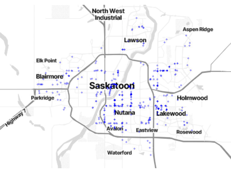
2.6 Section 6: Leisure activities
The following questions are used to generate the locations grouped into this section:
- Do you participate in any (individual or group) sports or leisure-time physical activities at least once per month?
- Do you visit a park at least once per month?
- Do you participate in or attend as a spectator a cultural or non-sport leisure activity at least once per month? For example: singing or drawing lessons, book or poker club, concert or play.
- Do you volunteer at least once per month?
- Do you engage in any religious or spiritual activities at least once per month?
- Do you go to a restaurant, café, bar or other food and drink establishment at least once per month?
- Do you get take-out food at least once per month?
- Do you regularly go for walks?
leisure_location <- locations[locations$location_category %in% c(17, 18, 19, 20, 21, 22, 23, 24), ] %>% dplyr::rename(location_category_code = location_category)
leisure_location$location_category <- factor(ifelse(leisure_location$location_category_code == 17, "17 [Leisure-time physical activity]",
  ifelse(leisure_location$location_category_code == 18, "18 [Park]",
    ifelse(leisure_location$location_category_code == 19, "19 [Cultural activity]",
      ifelse(leisure_location$location_category_code == 20, "20 [Volunteering place]",
        ifelse(leisure_location$location_category_code == 21, "21 [Religious or spiritual activity]",
          ifelse(leisure_location$location_category_code == 22, "22 [Restaurant, café, bar, etc. ]",
            ifelse(leisure_location$location_category_code == 23, "23 [Take-out]", "24 [Walk]")
          )
        )
      )
    )
  )
))

# map
bm + geom_sf(data = leisure_location, inherit.aes = FALSE, aes(color = location_category), size = 1.5, alpha = .3) +
  scale_color_brewer(palette = "Accent") +
  theme(legend.position = "bottom", legend.text = element_text(size = 8), legend.title = element_blank())
# compute number of shopping locations by category
ggplot(data = leisure_location) +
  geom_histogram(aes(x = location_category), stat = "count") +
  scale_x_discrete(labels = function(lbl) str_wrap(lbl, width = 20)) +
  labs(x = "Leisure locations by categories")
.location_category_cnt <- as.data.frame(leisure_location[c("location_category")]) %>%
  group_by(location_category) %>%
  dplyr::count() %>%
  arrange(location_category)
kable(.location_category_cnt, caption = "Shopping locations by categories") %>% kable_styling(bootstrap_options = "striped", full_width = T, position = "left")| location_category | n |
|---|---|
| 17 [Leisure-time physical activity] | 194 |
| 18 [Park] | 166 |
| 19 [Cultural activity] | 99 |
| 20 [Volunteering place] | 102 |
| 21 [Religious or spiritual activity] | 60 |
| 22 [Restaurant, café, bar, etc. ] | 401 |
| 23 [Take-out] | 200 |
| 24 [Walk] | 173 |
# compute statistics on shopping locations by participants and categories
# > one needs to account for participants who did not report location for some categories
.loc_iid_category_cnt <- as.data.frame(leisure_location[c("interact_id", "location_category")]) %>%
  group_by(interact_id, location_category) %>%
  dplyr::count()

# (cont'd) simulate SQL JOIN TABLE ON TRUE
.dummy <- data.frame(
  interact_iid = character(),
  location_category = character()
)
for (iid in as.vector(veritas_main$interact_id)) {
  .dmy <- distinct(.loc_iid_category_cnt[c("location_category")])
  .dmy$interact_id <- as.character(iid)
  .dummy <- rbind(.dummy, .dmy)
}

# (cont'd) find iid/categ combination without match in veritas locations
.no_leisure_iid <- dplyr::setdiff(.dummy, .loc_iid_category_cnt[c("location_category", "interact_id")]) %>%
  mutate(n = 0)

.loc_iid_category_cnt <- bind_rows(.loc_iid_category_cnt, .no_leisure_iid)

.location_category_cnt <- .loc_iid_category_cnt %>%
  group_by(location_category) %>%
  dplyr::summarise(min = min(n), mean = round(mean(n), 2), median = median(n), max = max(n)) %>%
  arrange(location_category)
kable(.location_category_cnt, caption = "Number of leisure locations by participant and category") %>% kable_styling(bootstrap_options = "striped", full_width = T, position = "left")| location_category | min | mean | median | max |
|---|---|---|---|---|
| 17 [Leisure-time physical activity] | 0 | 0.81 | 1 | 5 |
| 18 [Park] | 0 | 0.69 | 0 | 5 |
| 19 [Cultural activity] | 0 | 0.41 | 0 | 5 |
| 20 [Volunteering place] | 0 | 0.43 | 0 | 5 |
| 21 [Religious or spiritual activity] | 0 | 0.25 | 0 | 3 |
| 22 [Restaurant, café, bar, etc. ] | 0 | 1.68 | 1 | 5 |
| 23 [Take-out] | 0 | 0.84 | 0 | 5 |
| 24 [Walk] | 0 | 0.72 | 0 | 5 |
2.7 Section 7: Other places/activities
2.7.1 Are there other places that you go to at least once per month that we have not mentioned? For example: a mall, a daycare, a hardware store, or a community center.
# extract and recode
.other <- veritas_main[c("interact_id", "other")] %>% dplyr::rename(other_code = other)
.other$other <- factor(ifelse(.other$other_code == 1, "1 [Yes]",
  ifelse(.other$other_code == 2, "2 [No]", "N/A")
))

# histogram of answers
ggplot(data = .other) +
  geom_histogram(aes(x = other), stat = "count") +
  scale_x_discrete(labels = function(lbl) str_wrap(lbl, width = 20)) +
  labs(x = "other")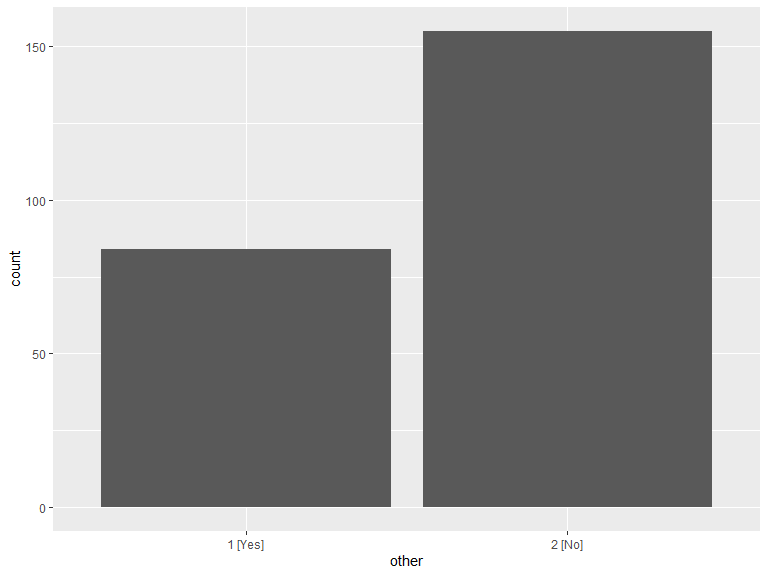
.other_cnt <- .other %>%
  group_by(other) %>%
  dplyr::count() %>%
  arrange(other)
kable(.other_cnt, caption = "Other places") %>% kable_styling(bootstrap_options = "striped", full_width = T, position = "left")| other | n |
|---|---|
| 1 [Yes] | 84 |
| 2 [No] | 155 |
2.7.2 Can you locate this place?
other_location <- locations[locations$location_category == 25, ]

bm + geom_sf(data = other_location, inherit.aes = FALSE, color = "blue", size = 1.8, alpha = .3)
2.8 Section 8: Areas of change
2.8.1 Can you locate areas where you have noticed an improvement of the urban environment?
# extract and recode
.improv <- veritas_main[c("interact_id", "improvement_none")] %>% dplyr::rename(improvement_none_code = improvement_none)
.improv$improvement_none <- factor(ifelse(.improv$improvement_none_code == 1, "1 [TRUE]",
  ifelse(.improv$improvement_none_code == 0, "0 [FALSE]", "N/A")
))

# histogram of answers
ggplot(data = .improv) +
  geom_histogram(aes(x = improvement_none), stat = "count") +
  scale_x_discrete(labels = function(lbl) str_wrap(lbl, width = 20)) +
  labs(x = "improvement_none")
.improv_cnt <- .improv %>%
  group_by(improvement_none) %>%
  dplyr::count() %>%
  arrange(improvement_none)
kable(.improv_cnt, caption = "No area of improvement") %>% kable_styling(bootstrap_options = "striped", full_width = T, position = "left")| improvement_none | n |
|---|---|
| 0 [FALSE] | 80 |
| 1 [TRUE] | 159 |
# polgon extraction
improv <- poly_geom[poly_geom$area_type == "improvement", ]

# Map
bm + geom_sf(data = improv, inherit.aes = FALSE, fill = alpha("blue", 0.3), color = alpha("blue", 0.5))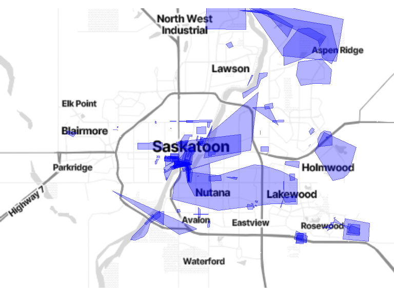
# Min, max, median & mean area of PRN
improv$area_m2 <- st_area(improv$geom)
kable(t(as.matrix(summary(improv$area_m2))),
  caption = "Area (in square meters) of the perceived improvement areas",
  digits = 1
) %>%
kable_styling(bootstrap_options = "striped", full_width = T, position = "left")| Min. | 1st Qu. | Median | Mean | 3rd Qu. | Max. |
|---|---|---|---|---|---|
| 274.5 | 49160.9 | 100759.6 | 905897.8 | 319319.5 | 17498425 |
2.8.2 Can you locate areas where you have noticed a deterioration of the urban environment?
# extract and recode
.deter <- veritas_main[c("interact_id", "deterioration_none")] %>% dplyr::rename(deterioration_none_code = deterioration_none)
.deter$deterioration_none <- factor(ifelse(.deter$deterioration_none_code == 1, "1 [TRUE]",
  ifelse(.deter$deterioration_none_code == 0, "0 [FALSE]", "N/A")
))

# histogram of answers
ggplot(data = .deter) +
  geom_histogram(aes(x = deterioration_none), stat = "count") +
  scale_x_discrete(labels = function(lbl) str_wrap(lbl, width = 20)) +
  labs(x = "deterioration_none")
.deter_cnt <- .deter %>%
  group_by(deterioration_none) %>%
  dplyr::count() %>%
  arrange(deterioration_none)
kable(.deter_cnt, caption = "No area of deterioration") %>% kable_styling(bootstrap_options = "striped", full_width = T, position = "left")| deterioration_none | n |
|---|---|
| 0 [FALSE] | 49 |
| 1 [TRUE] | 190 |
# polgon extraction
deter <- poly_geom[poly_geom$area_type == "deterioration", ]

# Map
bm + geom_sf(data = deter, inherit.aes = FALSE, fill = alpha("blue", 0.3), color = alpha("blue", 0.5))
# Min, max, median & mean area of PRN
deter$area_m2 <- st_area(deter$geom)
kable(t(as.matrix(summary(deter$area_m2))),
  caption = "Area (in square meters) of the perceived deterioration areas",
  digits = 1
) %>%
kable_styling(bootstrap_options = "striped", full_width = T, position = "left")| Min. | 1st Qu. | Median | Mean | 3rd Qu. | Max. |
|---|---|---|---|---|---|
| 240.7 | 21299.6 | 195864.1 | 1610266 | 889374.6 | 28113133 |
2.10 Derived metrics
2.10.1 Existence of improvement and deterioration areas by participant
Combination of improvement and/or deterioration areas per participant
# cross tab of improvement vs deteriation areas
.improv <- improv[c("interact_id")] %>%
  mutate(improv = "Improvement")
.deter <- deter[c("interact_id")] %>%
  mutate(deter = "Deterioration")
.ct_impr_deter <- veritas_main[c("interact_id")] %>%
  transmute(interact_id = as.character(interact_id)) %>%
  left_join(.improv, by = "interact_id") %>%
  left_join(.deter, by = "interact_id") %>%
  mutate_all(~ replace(., is.na(.), "N/A"))

kable(table(.ct_impr_deter$improv, .ct_impr_deter$deter), caption = "Improvement vs. deterioration") %>%
  kable_styling(bootstrap_options = "striped", full_width = T, position = "left", row_label_position = "r") %>%
column_spec(1, bold = T)| Deterioration | N/A | |
|---|---|---|
| Improvement | 30 | 43 |
| N/A | 16 | 150 |
2.10.2 Transportation mode preferences
Based on the answers to the question Usually, how do you go there? (Check all that apply.).
# code  en
# 1 By car and you drive
# 2 By car and someone else drives
# 3 By taxi/Uber
# 4 On foot
# 5 By bike
# 6 By bus
# 7 By subway
# 8 By train
# 99    Other

loc_labels <- data.frame(location_category = c(2:26), description = c(
  " 2 [Other residence]",
  " 3 [Work]",
  " 4 [School/College/University]",
  " 5 [Supermarket]",
  " 6 [Public/farmer’s market]",
  " 7 [Bakery]",
  " 8 [Specialty food store]",
  " 9 [Convenience store/Dépanneur]",
  "10 [Liquor store/SAQ]",
  "11 [Bank]",
  "12 [Hair salon/barbershop]",
  "13 [Post office]",
  "14 [Drugstore]",
  "15 [Doctor/healthcare provider]",
  "16 [Public transit stop]",
  "17 [Leisure-time physical activity]",
  "18 [Park]",
  "19 [Cultural activity]",
  "20 [Volunteering place]",
  "21 [Religious/spiritual activity]",
  "22 [Restaurant, café, bar, etc.]",
  "23 [Take-out]",
  "24 [Walk]",
  "25 [Other place]",
  "26 [Social contact residence]"
))

# extract and summary stats
.tm <- locations %>%
  st_set_geometry(NULL) %>%
  filter(location_category != 1) %>%
  left_join(loc_labels)

.tm_grouped <- .tm %>%
  group_by(description) %>%
  dplyr::summarise(
    N = n(), "By car (driver)" = sum(location_tmode_1),
    "By car (passenger)" = sum(location_tmode_2),
    "By taxi/Uber" = sum(location_tmode_3),
    "On foot" = sum(location_tmode_4),
    "By bike" = sum(location_tmode_5),
    "By bus" = sum(location_tmode_6),
    "Other" = sum(location_tmode_99)
  )

kable(.tm_grouped, caption = "Transportation mode preferences") %>% kable_styling(bootstrap_options = "striped", full_width = T, position = "left")| description | N | By car (driver) | By car (passenger) | By taxi/Uber | On foot | By bike | By bus | Other |
|---|---|---|---|---|---|---|---|---|
| 2 [Other residence] | 43 | 30 | 18 | 0 | 3 | 1 | 12 | 0 |
| 3 [Work] | 191 | 67 | 39 | 5 | 42 | 28 | 122 | 4 |
| 4 [School/College/University] | 141 | 28 | 21 | 1 | 44 | 17 | 117 | 1 |
| 5 [Supermarket] | 558 | 296 | 180 | 7 | 114 | 19 | 124 | 1 |
| 6 [Public/farmer’s market] | 59 | 26 | 12 | 0 | 22 | 13 | 13 | 0 |
| 7 [Bakery] | 48 | 24 | 10 | 0 | 24 | 5 | 7 | 0 |
| 8 [Specialty food store] | 82 | 32 | 20 | 0 | 34 | 9 | 19 | 0 |
| 9 [Convenience store/Dépanneur] | 153 | 50 | 14 | 0 | 82 | 8 | 33 | 0 |
| 10 [Liquor store/SAQ] | 137 | 76 | 34 | 5 | 40 | 6 | 21 | 0 |
| 11 [Bank] | 124 | 55 | 24 | 1 | 49 | 5 | 38 | 0 |
| 12 [Hair salon/barbershop] | 96 | 42 | 11 | 1 | 29 | 8 | 34 | 0 |
| 13 [Post office] | 91 | 35 | 13 | 0 | 50 | 11 | 29 | 0 |
| 14 [Drugstore] | 148 | 61 | 28 | 0 | 66 | 9 | 44 | 0 |
| 15 [Doctor/healthcare provider] | 195 | 82 | 37 | 6 | 30 | 9 | 97 | 0 |
| 16 [Public transit stop] | 439 | 6 | 3 | 0 | 418 | 3 | 0 | 19 |
| 17 [Leisure-time physical activity] | 194 | 94 | 39 | 0 | 63 | 19 | 48 | 1 |
| 18 [Park] | 166 | 11 | 19 | 0 | 131 | 31 | 9 | 2 |
| 19 [Cultural activity] | 99 | 40 | 41 | 7 | 39 | 12 | 28 | 0 |
| 20 [Volunteering place] | 102 | 35 | 27 | 0 | 44 | 13 | 35 | 3 |
| 21 [Religious/spiritual activity] | 60 | 26 | 24 | 2 | 21 | 5 | 15 | 1 |
| 22 [Restaurant, café, bar, etc.] | 401 | 150 | 145 | 14 | 162 | 40 | 78 | 1 |
| 23 [Take-out] | 200 | 71 | 60 | 1 | 37 | 5 | 23 | 46 |
| 24 [Walk] | 173 | 12 | 13 | 0 | 154 | 16 | 19 | 0 |
| 25 [Other place] | 147 | 70 | 40 | 3 | 40 | 11 | 46 | 0 |
# graph
.tm1 <- .tm %>%
  filter(location_tmode_1 == 1) %>%
  mutate(tm = "[1] By car (driver)")
.tm2 <- .tm %>%
  filter(location_tmode_2 == 1) %>%
  mutate(tm = "[2] By car (passenger)")
.tm3 <- .tm %>%
  filter(location_tmode_3 == 1) %>%
  mutate(tm = "[3] By taxi/Uber")
.tm4 <- .tm %>%
  filter(location_tmode_4 == 1) %>%
  mutate(tm = "[4] On foot")
.tm5 <- .tm %>%
  filter(location_tmode_5 == 1) %>%
  mutate(tm = "[5] By bike")
.tm6 <- .tm %>%
  filter(location_tmode_6 == 1) %>%
  mutate(tm = "[6] By bus")
.tm99 <- .tm %>%
  filter(location_tmode_99 == 1) %>%
  mutate(tm = "[99] Other")
.tm <- bind_rows(.tm1, .tm2) %>%
  bind_rows(.tm3) %>%
  bind_rows(.tm4) %>%
  bind_rows(.tm5) %>%
  bind_rows(.tm6) %>%
  bind_rows(.tm99)

# histogram of answers
ggplot(data = .tm) +
  geom_bar(aes(x = fct_rev(description), fill = tm), position = "fill") +
  scale_fill_brewer(palette = "Set3", name = "Transport modes") +
  scale_y_continuous(labels = percent) +
  labs(y = "Proportion of transportation mode by location category", x = element_blank()) +
  coord_flip() +
  theme(legend.position = "bottom", legend.justification = c(0, 0), legend.text = element_text(size = 8)) +
  guides(fill = guide_legend(nrow = 3))
2.10.3 Visiting places alone
Based on the answers to the question Do you usually go to this place alone or with other people?.
loc_labels <- data.frame(location_category = c(2:26), description = c(
  " 2 [Other residence]",
  " 3 [Work]",
  " 4 [School/College/University]",
  " 5 [Supermarket]",
  " 6 [Public/farmer’s market]",
  " 7 [Bakery]",
  " 8 [Specialty food store]",
  " 9 [Convenience store/Dépanneur]",
  "10 [Liquor store/SAQ]",
  "11 [Bank]",
  "12 [Hair salon/barbershop]",
  "13 [Post office]",
  "14 [Drugstore]",
  "15 [Doctor/healthcare provider]",
  "16 [Public transit stop]",
  "17 [Leisure-time physical activity]",
  "18 [Park]",
  "19 [Cultural activity]",
  "20 [Volunteering place]",
  "21 [Religious/spiritual activity]",
  "22 [Restaurant, café, bar, etc.]",
  "23 [Take-out]",
  "24 [Walk]",
  "25 [Other place]",
  "26 [Social contact residence]"
))

# extract and summary stats
.alone <- locations %>%
  st_set_geometry(NULL) %>%
  filter(location_category != 1) %>%
  left_join(loc_labels) %>%
  mutate(location_alone_recode = case_when(
    location_alone == 1 ~ 1,
    location_alone == 2 ~ 0
  ))

.alone_grouped <- .alone %>%
  group_by(description) %>%
  dplyr::summarise(
    N = n(), "Visited alone" = sum(location_alone_recode),
    "Visited alone (%)" = round(sum(location_alone_recode) * 100.0 / n(), digits = 1)
  )

kable(.alone_grouped, caption = "Visiting places alone") %>% kable_styling(bootstrap_options = "striped", full_width = T, position = "left")| description | N | Visited alone | Visited alone (%) |
|---|---|---|---|
| 2 [Other residence] | 43 | NA | NA |
| 3 [Work] | 191 | 61 | 31.9 |
| 4 [School/College/University] | 141 | 110 | 78.0 |
| 5 [Supermarket] | 558 | 316 | 56.6 |
| 6 [Public/farmer’s market] | 59 | 28 | 47.5 |
| 7 [Bakery] | 48 | 28 | 58.3 |
| 8 [Specialty food store] | 82 | 52 | 63.4 |
| 9 [Convenience store/Dépanneur] | 153 | 126 | 82.4 |
| 10 [Liquor store/SAQ] | 137 | 83 | 60.6 |
| 11 [Bank] | 124 | 101 | 81.5 |
| 12 [Hair salon/barbershop] | 96 | 88 | 91.7 |
| 13 [Post office] | 91 | 77 | 84.6 |
| 14 [Drugstore] | 148 | 119 | 80.4 |
| 15 [Doctor/healthcare provider] | 195 | 161 | 82.6 |
| 16 [Public transit stop] | 439 | 401 | 91.3 |
| 17 [Leisure-time physical activity] | 194 | 101 | 52.1 |
| 18 [Park] | 166 | 80 | 48.2 |
| 19 [Cultural activity] | 99 | 26 | 26.3 |
| 20 [Volunteering place] | 102 | 54 | 52.9 |
| 21 [Religious/spiritual activity] | 60 | 16 | 26.7 |
| 22 [Restaurant, café, bar, etc.] | 401 | 98 | 24.4 |
| 23 [Take-out] | 200 | 91 | 45.5 |
| 24 [Walk] | 173 | 101 | 58.4 |
| 25 [Other place] | 147 | 71 | 48.3 |
# histogram of answers
ggplot(data = .alone) +
  geom_bar(aes(x = fct_rev(description), fill = factor(location_alone)), position = "fill") +
  scale_fill_brewer(palette = "Set3", name = "Visiting places", labels = c("N/A", "Alone", "With someone")) +
  scale_y_continuous(labels = percent) +
  labs(y = "Proportion of places visited alone", x = element_blank()) +
  coord_flip()
2.10.4 Visit frequency
Based on the answers to the question How often do you go there?.
loc_labels <- data.frame(location_category = c(2:26), description = c(
  " 2 [Other residence]",
  " 3 [Work]",
  " 4 [School/College/University]",
  " 5 [Supermarket]",
  " 6 [Public/farmer’s market]",
  " 7 [Bakery]",
  " 8 [Specialty food store]",
  " 9 [Convenience store/Dépanneur]",
  "10 [Liquor store/SAQ]",
  "11 [Bank]",
  "12 [Hair salon/barbershop]",
  "13 [Post office]",
  "14 [Drugstore]",
  "15 [Doctor/healthcare provider]",
  "16 [Public transit stop]",
  "17 [Leisure-time physical activity]",
  "18 [Park]",
  "19 [Cultural activity]",
  "20 [Volunteering place]",
  "21 [Religious/spiritual activity]",
  "22 [Restaurant, café, bar, etc.]",
  "23 [Take-out]",
  "24 [Walk]",
  "25 [Other place]",
  "26 [Social contact residence]"
))

# extract and summary stats
.freq <- locations %>%
  st_set_geometry(NULL) %>%
  filter(location_category != 1) %>%
  left_join(loc_labels)

.freq_grouped <- .freq %>%
  group_by(description) %>%
  dplyr::summarise(
    N = n(), min = min(location_freq_visit),
    max = max(location_freq_visit),
    mean = mean(location_freq_visit),
    median = median(location_freq_visit),
    sd = sd(location_freq_visit)
  )

kable(.freq_grouped, caption = "Visit frequency (expressed in times/year)") %>% kable_styling(bootstrap_options = "striped", full_width = T, position = "left")| description | N | min | max | mean | median | sd |
|---|---|---|---|---|---|---|
| 2 [Other residence] | 43 | 6 | 364 | 108.976744 | 104 | 89.169044 |
| 3 [Work] | 191 | 2 | 416 | 190.963351 | 240 | 93.326556 |
| 4 [School/College/University] | 141 | 1 | 1040 | 245.014184 | 260 | 132.401877 |
| 5 [Supermarket] | 558 | 0 | 312 | 42.603943 | 24 | 45.243516 |
| 6 [Public/farmer’s market] | 59 | 3 | 156 | 26.525424 | 24 | 24.614515 |
| 7 [Bakery] | 48 | 1 | 104 | 30.104167 | 24 | 24.121360 |
| 8 [Specialty food store] | 82 | 2 | 104 | 21.073171 | 12 | 17.760951 |
| 9 [Convenience store/Dépanneur] | 153 | 2 | 520 | 53.196078 | 36 | 70.149564 |
| 10 [Liquor store/SAQ] | 137 | 2 | 156 | 19.481752 | 12 | 19.082677 |
| 11 [Bank] | 124 | 1 | 104 | 16.774193 | 12 | 18.283156 |
| 12 [Hair salon/barbershop] | 96 | 1 | 36 | 7.281250 | 6 | 5.495842 |
| 13 [Post office] | 91 | 1 | 208 | 18.560440 | 8 | 33.004784 |
| 14 [Drugstore] | 148 | 4 | 260 | 28.445946 | 12 | 37.854948 |
| 15 [Doctor/healthcare provider] | 195 | 1 | 96 | 6.917949 | 4 | 9.287140 |
| 16 [Public transit stop] | 439 | 0 | 1040 | 195.560364 | 156 | 173.685790 |
| 17 [Leisure-time physical activity] | 194 | 1 | 364 | 94.360825 | 52 | 83.703113 |
| 18 [Park] | 166 | 2 | 728 | 77.873494 | 52 | 95.502827 |
| 19 [Cultural activity] | 99 | 1 | 260 | 30.646465 | 12 | 48.635737 |
| 20 [Volunteering place] | 102 | 1 | 364 | 81.401961 | 51 | 104.069309 |
| 21 [Religious/spiritual activity] | 60 | 12 | 364 | 73.400000 | 52 | 84.666685 |
| 22 [Restaurant, café, bar, etc.] | 401 | 1 | 260 | 30.932668 | 12 | 43.392948 |
| 23 [Take-out] | 200 | 0 | 260 | 23.345000 | 12 | 36.191645 |
| 24 [Walk] | 173 | 2 | 728 | 109.705202 | 52 | 109.373904 |
| 25 [Other place] | 147 | 1 | 520 | 50.795918 | 24 | 75.428542 |
# graph
ggplot(data = .freq) +
  geom_boxplot(aes(x = fct_rev(description), y = location_freq_visit)) +
  scale_y_continuous(limits = c(0, 365)) +
  labs(y = "Visits/year (Frequency over 1 visit/day not shown)", x = element_blank()) +
  coord_flip()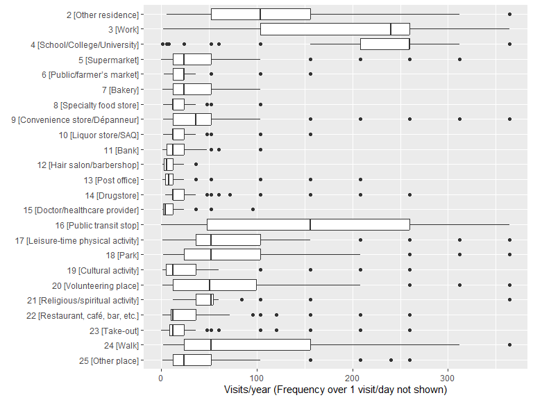
2.10.5 Spatial indicators: Camille Perchoux’s toolbox
Below is a list of indicators proposed by Camille Perchoux in her paper Assessing patterns of spatial behavior in health studies: Their socio-demographic determinants and associations with transportation modes (the RECORD Cohort Study).
-- Reading Camille tbx indics from Essence table
SELECT interact_id,
  n_acti_places, n_weekly_vst, n_acti_types,
  cvx_perimeter, cvx_surface,
  min_length, max_length, median_length,
  pct_visits_neighb,
  n_acti_prn, pct_visits_prn, prn_area_km2
FROM essence_table.essence_perchoux_tbx
WHERE city_id = 'Saskatoon' AND wave_id = 1

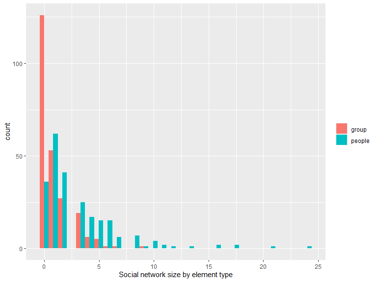
2.10.6 Social indicators: Alexandre Naud’s toolbox
See Alex’s document for a more comprehensive presentation of the social indicators.
2.10.6.1 Number of people in the network (
people_degree)2.10.6.2 Simmelian Brokerage (
simmelian)2.10.6.3 Number of people with whom the participant like to socialize (
socialize_size)2.10.6.4 Weekly face-to-face interactions among people with whom the participant like to socialize (
socialize_meet)2.10.6.5 Weekly ICT interactions among people with whom the participant like to socialize (
socialize_chat)2.10.6.6 Number of people with whom the participant discuss important matters (
important_size)2.10.6.7 Number of people in all groups (
group_degree)