INTERACT Saskatoon Participant VERITAS Summary - W2 - new and returning

1 VERITAS dataset description

Unlike the Eligibility or Health questionnaires, which can mostly be encoded as a flat table, the VERITAS questionnaire implicitly records a series of entities and their relationships:

• Places: list of geocoded locations visited by participants, along with the following characteristics: category, name, visit frequency, transportation mode
• Social contacts: people and/or groups frequented by participants
• Relationships: between social contacts (who knows who / who belongs to which group) as well as between locations and social contacts (places visited along with whom)

The diagram below illustrates the various entities collected throught the VERITAS questionnaire:

VERITAS entities

New participants and returning participants are presented separately below, as they were presented two slightly different question flows.

2 Basic descriptive statistics for new participants

2.1 Section 1: Residence and Neighbourhood

2.1.1 Now, let’s start with your home. What is your address?

home_location <- locations[locations$location_category == 1, ]

## version ggmap
skt_aoi <- st_bbox(home_location)
names(skt_aoi) <- c("left", "bottom", "right", "top")
skt_aoi[["left"]] <- skt_aoi[["left"]] - .07
skt_aoi[["right"]] <- skt_aoi[["right"]] + .07
skt_aoi[["top"]] <- skt_aoi[["top"]] + .01
skt_aoi[["bottom"]] <- skt_aoi[["bottom"]] - .01

bm <- get_stadiamap(skt_aoi, zoom = 11, maptype = "stamen_toner_lite") %>%
  ggmap(extent = "device")
bm + geom_sf(data = st_jitter(home_location, .008), inherit.aes = FALSE, color = "blue", size = 1.8, alpha = .3) # see https://github.com/r-spatial/sf/issues/336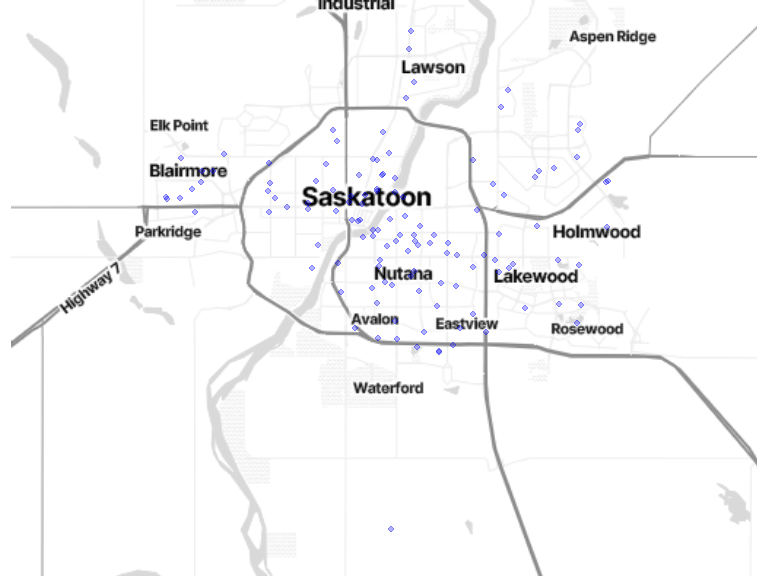

NB: Home locations have been randomly shifted from their original position to protect privacy.

# Number of participants by municipalites
home_by_municipalites <- st_join(home_location, municipalities["NAME"])
home_by_mun_cnt <- as.data.frame(home_by_municipalites) %>%
  group_by(NAME) %>%
  dplyr::count() %>%
  arrange(desc(n), NAME)
home_by_mun_cnt$Shape <- NULL
kable(home_by_mun_cnt, caption = "Number of participants by municipalities") %>% kable_styling(bootstrap_options = "striped", full_width = T, position = "left")

Number of participants by municipalities

NAME	n
Saskatoon	123
Corman Park	1

2.1.2 If you were asked to draw the boundaries of your neighbourhood, what would they be?

prn <- poly_geom[poly_geom$area_type == "neighborhood", ]

## version ggmap
bm + geom_sf(data = prn, inherit.aes = FALSE, fill = alpha("blue", 0.05), color = alpha("blue", 0.3))

# Min, max, median & mean area of PRN
prn$area_m2 <- st_area(prn$geom)
kable(t(as.matrix(summary(prn$area_m2))),
  caption = "Area (in square meters) of the perceived residential neighborhood",
  digits = 1
) %>%
  kable_styling(bootstrap_options = "striped", full_width = T, position = "left")

Area (in square meters) of the perceived residential neighborhood

Min.	1st Qu.	Median	Mean	3rd Qu.	Max.
4959.1	272957.2	742214.6	1050349	1432838	6363390

NB only 110 valid neighborhoods were collected, as many participants struggled to draw polygons on the map.

2.1.3 How attached are you to your neighbourhood?

# extract and recode
.ngh_att <- veritas_main[veritas_main$neighbourhood_attach != 99, c("interact_id", "neighbourhood_attach")] %>% dplyr::rename(neighbourhood_attach_code = neighbourhood_attach)
.ngh_att$neighbourhood_attach <- factor(ifelse(.ngh_att$neighbourhood_attach_code == 1, "1 [Not attached at all]",
  ifelse(.ngh_att$neighbourhood_attach_code == 6, "6 [Very attached]",
    .ngh_att$neighbourhood_attach_code
  )
))

# histogram of attachment
ggplot(data = .ngh_att) +
  geom_histogram(aes(x = neighbourhood_attach), stat = "count") +
  scale_x_discrete(labels = function(lbl) str_wrap(lbl, width = 20)) +
  labs(x = "neighbourhood_attach")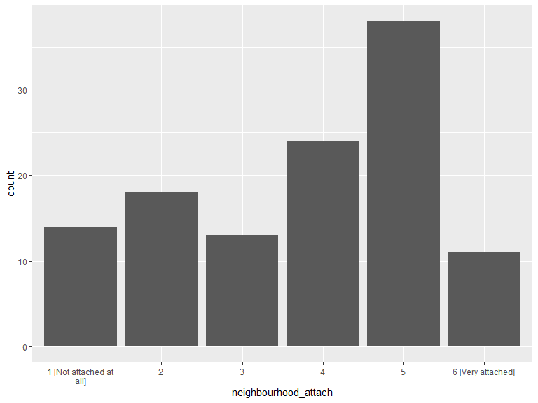

.ngh_att_cnt <- .ngh_att %>%
  group_by(neighbourhood_attach) %>%
  dplyr::count() %>%
  arrange(neighbourhood_attach)
kable(.ngh_att_cnt, caption = "Neigbourhood attachment") %>% 
  kable_styling(bootstrap_options = "striped", full_width = T, position = "left")

Neigbourhood attachment

neighbourhood_attach	n
1 [Not attached at all]	14
2	18
3	13
4	24
5	38
6 [Very attached]	11

2.1.4 On average, how many hours per day do you spend outside of your home?

# histogram of n hours out
ggplot(data = veritas_main) +
  geom_histogram(aes(x = hours_out))

# Min, max, median & mean hours/day out
kable(t(as.matrix(summary(veritas_main$hours_out))),
  caption = "Hours/day outside home",
  digits = 1
) %>%
  kable_styling(bootstrap_options = "striped", full_width = T, position = "left")

Hours/day outside home

Min.	1st Qu.	Median	Mean	3rd Qu.	Max.
1	2	4	5.7	9	24

2.1.5 Of this time spent outside your home, on average how many hours do you spend outside your neighbourhood?

# histogram of n hours out
ggplot(data = veritas_main) +
  geom_histogram(aes(x = hours_out_neighb))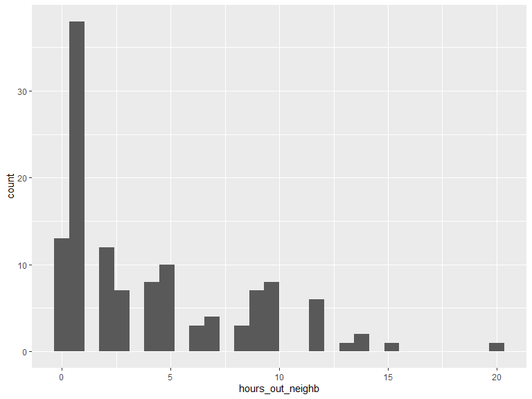

# Min, max, median & mean hours/day out of neighborhood
kable(t(as.matrix(summary(veritas_main$hours_out_neighb))),
  caption = "Hours/day outside neighbourhood",
  digits = 1
) %>%
  kable_styling(bootstrap_options = "striped", full_width = T, position = "left")

Hours/day outside neighbourhood

Min.	1st Qu.	Median	Mean	3rd Qu.	Max.
0	1	2	4.2	7	20

2.1.6 Are there one or more areas close to where you live that you tend to avoid because you do not feel safe there (for any reason)?

# extract and recode
.unsafe <- veritas_main[c("interact_id", "unsafe_area")] %>% dplyr::rename(unsafe_area_code = unsafe_area)
.unsafe$unsafe_area <- factor(ifelse(.unsafe$unsafe_area_code == 1, "1 [Yes]",
  ifelse(.unsafe$unsafe_area_code == 2, "2 [No]", "N/A")
))

# histogram of answers
ggplot(data = .unsafe) +
  geom_histogram(aes(x = unsafe_area), stat = "count") +
  scale_x_discrete(labels = function(lbl) str_wrap(lbl, width = 20)) +
  labs(x = "unsafe_area")

.unsafe_cnt <- .unsafe %>%
  group_by(unsafe_area) %>%
  dplyr::count() %>%
  arrange(unsafe_area)
kable(.unsafe_cnt, caption = "Unsafe areas") %>% kable_styling(bootstrap_options = "striped", full_width = T, position = "left")

Unsafe areas

unsafe_area	n
1 [Yes]	30
2 [No]	94

# map
unsafe <- poly_geom[poly_geom$area_type == "unsafe area", ]

## version ggmap
bm + geom_sf(data = unsafe, inherit.aes = FALSE, fill = alpha("blue", 0.3), color = alpha("blue", 0.5))

# Min, max, median & mean area of PRN
unsafe$area_m2 <- st_area(unsafe$geom)
kable(t(as.matrix(summary(unsafe$area_m2))),
  caption = "Area (in square meters) of the perceived unsafe area",
  digits = 1
) %>%
  kable_styling(bootstrap_options = "striped", full_width = T, position = "left")

Area (in square meters) of the perceived unsafe area

Min.	1st Qu.	Median	Mean	3rd Qu.	Max.
1345.1	54800.9	256594.1	3632394	1809054	68822075

2.1.7 Do you spend the night somewhere other than your home at least once per week?

# extract and recode
.o_res <- veritas_main[c("interact_id", "other_resid")] %>% dplyr::rename(other_resid_code = other_resid)
.o_res$other_resid <- factor(ifelse(.o_res$other_resid_code == 1, "1 [Yes]",
  ifelse(.o_res$other_resid_code == 2, "2 [No]", "N/A")
))

# histogram of answers
ggplot(data = .o_res) +
  geom_histogram(aes(x = other_resid), stat = "count") +
  scale_x_discrete(labels = function(lbl) str_wrap(lbl, width = 20)) +
  labs(x = "other_resid")

.o_res_cnt <- .o_res %>%
  group_by(other_resid) %>%
  dplyr::count() %>%
  arrange(other_resid)
kable(.o_res_cnt, caption = "Other residence") %>% kable_styling(bootstrap_options = "striped", full_width = T, position = "left")

Other residence

other_resid	n
1 [Yes]	18
2 [No]	106

2.2 Section 2: Occupation

2.2.1 Are you currently working?

# extract and recode
.work <- veritas_main[c("interact_id", "working")] %>% dplyr::rename(working_code = working)
.work$working <- factor(ifelse(.work$working_code == 1, "1 [Yes]",
  ifelse(.work$working_code == 2, "2 [No]", "N/A")
))

# histogram of answers
ggplot(data = .work) +
  geom_histogram(aes(x = working), stat = "count") +
  scale_x_discrete(labels = function(lbl) str_wrap(lbl, width = 20)) +
  labs(x = "working")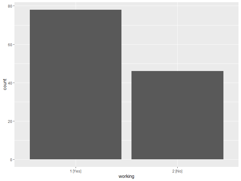

.work_cnt <- .work %>%
  group_by(working) %>%
  dplyr::count() %>%
  arrange(working)
kable(.work_cnt, caption = "Currently working") %>% 
  kable_styling(bootstrap_options = "striped", full_width = T, position = "left")

Currently working

working	n
1 [Yes]	78
2 [No]	46

2.2.2 Where do you work?

work_location <- locations[locations$location_category == 3, ]

bm + geom_sf(data = work_location, inherit.aes = FALSE, color = "blue", size = 1.8, alpha = .3)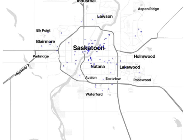

2.2.3 On average, how many hours per week do you work?

# histogram of n hours out
ggplot(data = veritas_main[veritas_main$working == 1, ]) +
  geom_histogram(aes(x = work_hours))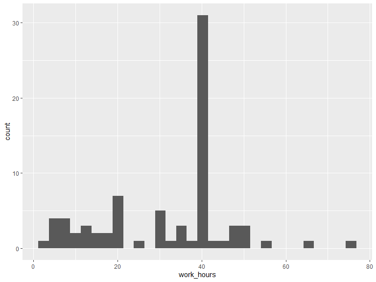

# Min, max, median & mean hours/day out
kable(t(as.matrix(summary(veritas_main$work_hours[veritas_main$working == 1]))),
  caption = "Work hours/week",
  digits = 1
) %>%
  kable_styling(bootstrap_options = "striped", full_width = T, position = "left")

Work hours/week

Min.	1st Qu.	Median	Mean	3rd Qu.	Max.
2	20	40	31.8	40	75

2.2.4 Are you currently a registered student?

# extract and recode
.study <- veritas_main[c("interact_id", "studying")] %>% dplyr::rename(studying_code = studying)
.study$studying <- factor(ifelse(.study$studying_code == 1, "1 [Yes]",
  ifelse(.study$studying_code == 2, "2 [No]", "N/A")
))

# histogram of answers
ggplot(data = .study) +
  geom_histogram(aes(x = studying), stat = "count") +
  scale_x_discrete(labels = function(lbl) str_wrap(lbl, width = 20)) +
  labs(x = "Studying")

.study_cnt <- .study %>%
  group_by(studying) %>%
  dplyr::count() %>%
  arrange(studying)
kable(.study_cnt, caption = "Currently studying") %>% kable_styling(bootstrap_options = "striped", full_width = T, position = "left")

Currently studying

studying	n
1 [Yes]	45
2 [No]	79

2.2.5 Where do you study?

study_location <- locations[locations$location_category == 4, ]

bm + geom_sf(data = study_location, inherit.aes = FALSE, color = "blue", size = 1.8, alpha = .3)

2.2.6 On average, how many hours per week do you study?

# histogram of n hours out
ggplot(data = veritas_main[veritas_main$studying == 1, ]) +
  geom_histogram(aes(x = study_hours))

# Min, max, median & mean hours/day out
kable(t(as.matrix(summary(veritas_main$study_hours[veritas_main$studying == 1]))),
  caption = "study hours/week",
  digits = 1
) %>%
  kable_styling(bootstrap_options = "striped", full_width = T, position = "left")

study hours/week

Min.	1st Qu.	Median	Mean	3rd Qu.	Max.
4	15	30	29.1	40	70

2.3 Section 3: Shopping activities

The following questions are used to generate the locations grouped into this section:

1. Do you shop for groceries at a supermarket at least once per month?
2. Do you shop at a public/farmer’s market at least once per month?
3. Do you shop at a bakery at least once per month?
4. Do you go to a specialty food store at least once per month? For example: a cheese shop, fruit and vegetable store, butcher’s shop, natural and health food store.
5. Do you go to a convenience store at least once per month?
6. Do you go to a liquor store at least once per month?

shop_lut <- data.frame(
  location_category_code = c(5, 6, 7, 8, 9, 10),
  location_category = factor(c(
    " 5 [Supermarket]",
    " 6 [Public/farmer’s market]",
    " 7 [Bakery]",
    " 8 [Specialty food store]",
    " 9 [Convenience store/Dépanneur]",
    "10 [Liquor store/SAQ]"
  ))
)
shop_location <- locations[locations$location_category %in% shop_lut$location_category_code, ] %>%
  dplyr::rename(location_category_code = location_category) %>%
  inner_join(shop_lut, by = "location_category_code")

# map
bm + geom_sf(data = shop_location, inherit.aes = FALSE, aes(color = location_category), size = 1.5, alpha = .3) +
  scale_color_brewer(palette = "Accent") +
  theme(legend.position = "bottom", legend.text = element_text(size = 8), legend.title = element_blank())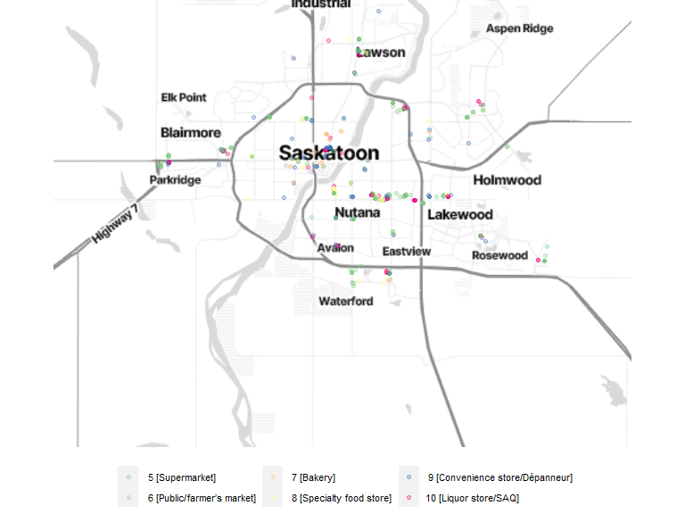

# compute number of shopping locations by category
ggplot(data = shop_location) +
  geom_histogram(aes(x = location_category), stat = "count") +
  scale_x_discrete(labels = function(lbl) str_wrap(lbl, width = 20)) +
  labs(x = "Shopping locations by categories")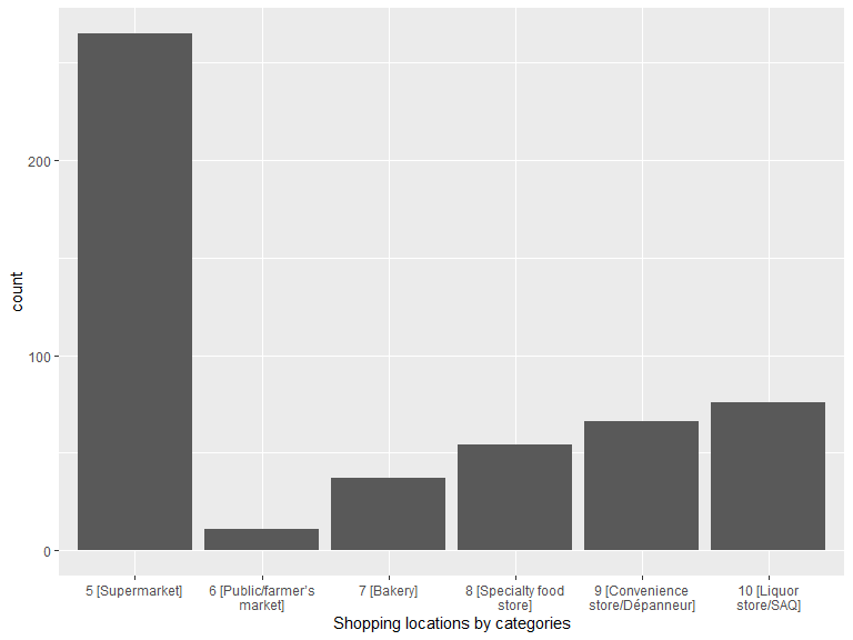

.location_category_cnt <- as.data.frame(shop_location[c("location_category")]) %>%
  group_by(location_category) %>%
  dplyr::count() %>%
  arrange(location_category)
kable(.location_category_cnt, caption = "Shopping locations by categories") %>% kable_styling(bootstrap_options = "striped", full_width = T, position = "left")

Shopping locations by categories

location_category	n
5 [Supermarket]	265
6 [Public/farmer’s market]	11
7 [Bakery]	37
8 [Specialty food store]	54
9 [Convenience store/Dépanneur]	66
10 [Liquor store/SAQ]	76

# compute statistics on shopping locations by participants and categories
# > one needs to account for participants who did not report location for some categories
.loc_iid_category_cnt <- as.data.frame(shop_location[c("interact_id", "location_category")]) %>%
  group_by(interact_id, location_category) %>%
  dplyr::count()

# (cont'd) simulate SQL JOIN TABLE ON TRUE to build list of all combination iid/shopping categ
.dummy <- data_frame(
  interact_id = character(),
  location_category = character()
)
for (iid in as.vector(veritas_main$interact_id)) {
  .dmy <- data_frame(
    interact_id = as.character(iid),
    location_category = shop_lut$location_category
  )
  .dummy <- rbind(.dummy, .dmy)
}

# (cont'd) find iid/categ combination without match in veritas locations
.no_shop_iid <- dplyr::setdiff(.dummy, .loc_iid_category_cnt[c("location_category", "interact_id")]) %>%
  mutate(n = 0)
.loc_iid_category_cnt <- bind_rows(.loc_iid_category_cnt, .no_shop_iid)

.location_category_cnt <- .loc_iid_category_cnt %>%
  group_by(location_category) %>%
  dplyr::summarise(min = min(n), mean = round(mean(n), 2), median = median(n), max = max(n)) %>%
  arrange(location_category)
kable(.location_category_cnt, caption = "Number of shopping locations by participant and category") %>% kable_styling(bootstrap_options = "striped", full_width = T, position = "left")

Number of shopping locations by participant and category

location_category	min	mean	median	max
5 [Supermarket]	0	2.14	2	5
6 [Public/farmer’s market]	0	0.09	0	2
7 [Bakery]	0	0.30	0	4
8 [Specialty food store]	0	0.44	0	4
9 [Convenience store/Dépanneur]	0	0.53	0	4
10 [Liquor store/SAQ]	0	0.61	0	4

2.4 Section 4: Services

The following questions are used to generate the locations grouped into this section:

1. Where is the bank you go to most often located?
2. Where is the hair salon or barber shop you go to most often?
3. Where is the post office where you go to most often?
4. Where is the drugstore you go to most often?
5. If you need to visit a doctor or other healthcare provider, where do you go most often?

serv_lut <- data.frame(
  location_category_code = c(11, 12, 13, 14, 15),
  location_category = factor(c(
    "11 [Bank]",
    "12 [Hair salon/barbershop]",
    "13 [Post office]",
    "14 [Drugstore]",
    "15 [Doctor/healthcare provider]"
  ))
)
serv_location <- locations[locations$location_category %in% serv_lut$location_category_code, ] %>%
  dplyr::rename(location_category_code = location_category) %>%
  inner_join(serv_lut, by = "location_category_code")

# map
bm + geom_sf(data = serv_location, inherit.aes = FALSE, aes(color = location_category), size = 1.5, alpha = .3) +
  scale_color_brewer(palette = "Accent") +
  theme(legend.position = "bottom", legend.text = element_text(size = 8), legend.title = element_blank())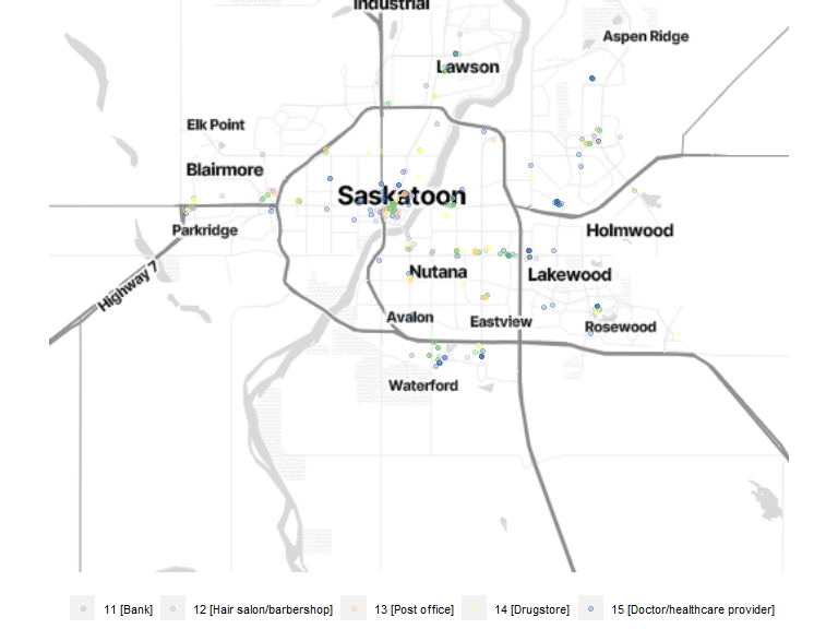

# compute number of shopping locations by category
ggplot(data = serv_location) +
  geom_histogram(aes(x = location_category), stat = "count") +
  scale_x_discrete(labels = function(lbl) str_wrap(lbl, width = 20)) +
  labs(x = "Service locations by categories")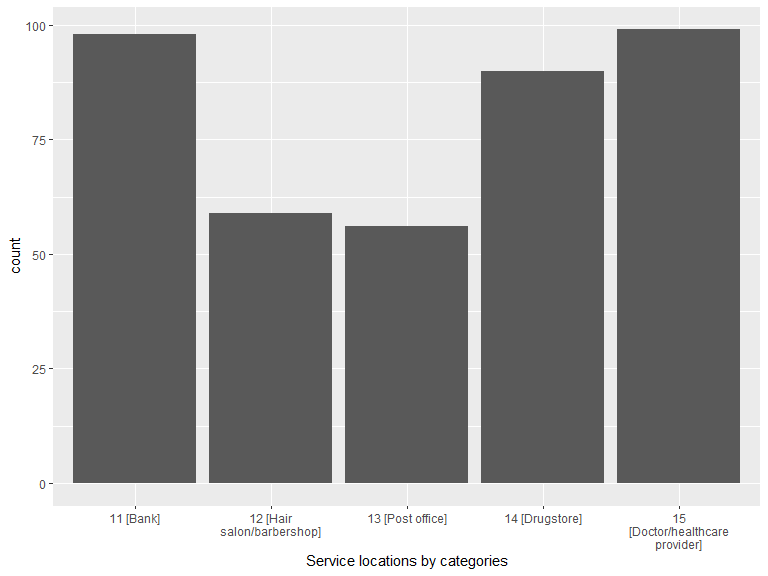

.location_category_cnt <- as.data.frame(serv_location[c("location_category")]) %>%
  group_by(location_category) %>%
  dplyr::count() %>%
  arrange(location_category)
kable(.location_category_cnt, caption = "Shopping locations by categories") %>% kable_styling(bootstrap_options = "striped", full_width = T, position = "left")

Shopping locations by categories

location_category	n
11 [Bank]	98
12 [Hair salon/barbershop]	59
13 [Post office]	56
14 [Drugstore]	90
15 [Doctor/healthcare provider]	99

# compute statistics on shopping locations by participants and categories
# > one needs to account for participants who did not report location for some categories
.loc_iid_category_cnt <- as.data.frame(serv_location[c("interact_id", "location_category")]) %>%
  group_by(interact_id, location_category) %>%
  dplyr::count()

# (cont'd) simulate SQL JOIN TABLE ON TRUE
.dummy <- data_frame(
  interact_id = character(),
  location_category = character()
)
for (iid in as.vector(veritas_main$interact_id)) {
  .dmy <- data_frame(
    interact_id = as.character(iid),
    location_category = serv_lut$location_category
  )
  .dummy <- rbind(.dummy, .dmy)
}

# (cont'd) find iid/categ combination without match in veritas locations
.no_serv_iid <- dplyr::setdiff(.dummy, .loc_iid_category_cnt[c("location_category", "interact_id")]) %>%
  mutate(n = 0)
.loc_iid_category_cnt <- bind_rows(.loc_iid_category_cnt, .no_serv_iid)

.location_category_cnt <- .loc_iid_category_cnt %>%
  group_by(location_category) %>%
  dplyr::summarise(min = min(n), mean = round(mean(n), 2), median = median(n), max = max(n)) %>%
  arrange(location_category)
kable(.location_category_cnt, caption = "Number of shopping locations by participant and category") %>% kable_styling(bootstrap_options = "striped", full_width = T, position = "left")

Number of shopping locations by participant and category

location_category	min	mean	median	max
11 [Bank]	0	0.79	1	1
12 [Hair salon/barbershop]	0	0.48	0	1
13 [Post office]	0	0.45	0	1
14 [Drugstore]	0	0.73	1	1
15 [Doctor/healthcare provider]	0	0.80	1	5

2.5 Section 5: Transportation

2.5.1 Do you use public transit from your home?

# extract and recode
.transp <- veritas_main[c("interact_id", "public_transit")] %>% dplyr::rename(public_transit_code = public_transit)
.transp$public_transit <- factor(ifelse(.transp$public_transit_code == 1, "1 [Yes]",
  ifelse(.transp$public_transit_code == 2, "2 [No]", "N/A")
))

# histogram of answers
ggplot(data = .transp) +
  geom_histogram(aes(x = public_transit), stat = "count") +
  scale_x_discrete(labels = function(lbl) str_wrap(lbl, width = 20)) +
  labs(x = "public_transit")

.transp_cnt <- .transp %>%
  group_by(public_transit) %>%
  dplyr::count() %>%
  arrange(public_transit)
kable(.transp_cnt, caption = "Use public transit") %>% kable_styling(bootstrap_options = "striped", full_width = T, position = "left")

Use public transit

public_transit	n
1 [Yes]	62
2 [No]	62

2.5.2 Where are the public transit stops that you access from your home?

transp_location <- locations[locations$location_category == 16, ]

bm + geom_sf(data = transp_location, inherit.aes = FALSE, color = "blue", size = 1.8, alpha = .3)

2.6 Section 6: Leisure activities

The following questions are used to generate the locations grouped into this section:

1. Do you participate in any (individual or group) sports or leisure-time physical activities at least once per month?
2. Do you visit a park at least once per month?
3. Do you participate in or attend as a spectator a cultural or non-sport leisure activity at least once per month? For example: singing or drawing lessons, book or poker club, concert or play.
4. Do you volunteer at least once per month?
5. Do you engage in any religious or spiritual activities at least once per month?
6. Do you go to a restaurant, café, bar or other food and drink establishment at least once per month?
7. Do you get take-out food at least once per month?
8. Do you regularly go for walks?

leisure_lut <- data.frame(
  location_category_code = c(17, 18, 19, 20, 21, 22, 23, 24),
  location_category = factor(c(
    "17 [Leisure-time physical activity]",
    "18 [Park]",
    "19 [Cultural activity]",
    "20 [Volunteering place]",
    "21 [Religious or spiritual activity]",
    "22 [Restaurant, café, bar, etc. ]",
    "23 [Take-out]",
    "24 [Walk]"
  ))
)
leisure_location <- locations[locations$location_category %in% leisure_lut$location_category_code, ] %>%
  dplyr::rename(location_category_code = location_category) %>%
  inner_join(leisure_lut, by = "location_category_code")

# map
bm + geom_sf(data = leisure_location, inherit.aes = FALSE, aes(color = location_category), size = 1.5, alpha = .3) +
  scale_color_brewer(palette = "Accent") +
  theme(legend.position = "bottom", legend.text = element_text(size = 8), legend.title = element_blank())

# compute number of shopping locations by category
ggplot(data = leisure_location) +
  geom_histogram(aes(x = location_category), stat = "count") +
  scale_x_discrete(labels = function(lbl) str_wrap(lbl, width = 20)) +
  labs(x = "Leisure locations by categories")

.location_category_cnt <- as.data.frame(leisure_location[c("location_category")]) %>%
  group_by(location_category) %>%
  dplyr::count() %>%
  arrange(location_category)
kable(.location_category_cnt, caption = "Shopping locations by categories") %>% kable_styling(bootstrap_options = "striped", full_width = T, position = "left")

Shopping locations by categories

location_category	n
17 [Leisure-time physical activity]	76
18 [Park]	112
19 [Cultural activity]	1
20 [Volunteering place]	15
21 [Religious or spiritual activity]	11
22 [Restaurant, café, bar, etc. ]	123
23 [Take-out]	151
24 [Walk]	131

# compute statistics on shopping locations by participants and categories
# > one needs to account for participants who did not report location for some categories
.loc_iid_category_cnt <- as.data.frame(leisure_location[c("interact_id", "location_category")]) %>%
  group_by(interact_id, location_category) %>%
  dplyr::count()

# (cont'd) simulate SQL JOIN TABLE ON TRUE
.dummy <- data_frame(
  interact_id = character(),
  location_category = character()
)
for (iid in as.vector(veritas_main$interact_id)) {
  .dmy <- data_frame(
    interact_id = as.character(iid),
    location_category = leisure_lut$location_category
  )
  .dummy <- rbind(.dummy, .dmy)
}

# (cont'd) find iid/categ combination without match in veritas locations
.no_leisure_iid <- dplyr::setdiff(.dummy, .loc_iid_category_cnt[c("location_category", "interact_id")]) %>%
  mutate(n = 0)

.loc_iid_category_cnt <- bind_rows(.loc_iid_category_cnt, .no_leisure_iid)

.location_category_cnt <- .loc_iid_category_cnt %>%
  group_by(location_category) %>%
  dplyr::summarise(min = min(n), mean = round(mean(n), 2), median = median(n), max = max(n)) %>%
  arrange(location_category)
kable(.location_category_cnt, caption = "Number of leisure locations by participant and category") %>% kable_styling(bootstrap_options = "striped", full_width = T, position = "left")

Number of leisure locations by participant and category

location_category	min	mean	median	max
17 [Leisure-time physical activity]	0	0.61	0	5
18 [Park]	0	0.90	1	5
19 [Cultural activity]	0	0.01	0	1
20 [Volunteering place]	0	0.12	0	1
21 [Religious or spiritual activity]	0	0.09	0	3
22 [Restaurant, café, bar, etc. ]	0	0.99	1	5
23 [Take-out]	0	1.22	1	5
24 [Walk]	0	1.06	1	5

2.7 Section 7: Other places/activities

2.7.1 Are there other places that you go to at least once per month that we have not mentioned? For example: a mall, a daycare, a hardware store, or a community center.

# extract and recode
.other <- veritas_main[c("interact_id", "other")] %>% dplyr::rename(other_code = other)
.other$other <- factor(ifelse(.other$other_code == 1, "1 [Yes]",
  ifelse(.other$other_code == 2, "2 [No]", "N/A")
))

# histogram of answers
ggplot(data = .other) +
  geom_histogram(aes(x = other), stat = "count") +
  scale_x_discrete(labels = function(lbl) str_wrap(lbl, width = 20)) +
  labs(x = "other")

.other_cnt <- .other %>%
  group_by(other) %>%
  dplyr::count() %>%
  arrange(other)
kable(.other_cnt, caption = "Other places") %>% kable_styling(bootstrap_options = "striped", full_width = T, position = "left")

Other places

other	n
1 [Yes]	24
2 [No]	100

2.7.2 Can you locate this place?

other_location <- locations[locations$location_category == 25, ]

bm + geom_sf(data = other_location, inherit.aes = FALSE, color = "blue", size = 1.8, alpha = .3)

2.8 Section 8: Areas of change

2.8.1 Can you locate areas where you have noticed an improvement of the urban environment?

# extract and recode
.improv <- veritas_main[c("interact_id", "improvement_none")] %>% dplyr::rename(improvement_none_code = improvement_none)
.improv$improvement_none <- factor(ifelse(.improv$improvement_none_code == 1, "1 [TRUE]",
  ifelse(.improv$improvement_none_code == 0, "0 [FALSE]", "N/A")
))

# histogram of answers
ggplot(data = .improv) +
  geom_histogram(aes(x = improvement_none), stat = "count") +
  scale_x_discrete(labels = function(lbl) str_wrap(lbl, width = 20)) +
  labs(x = "improvement_none")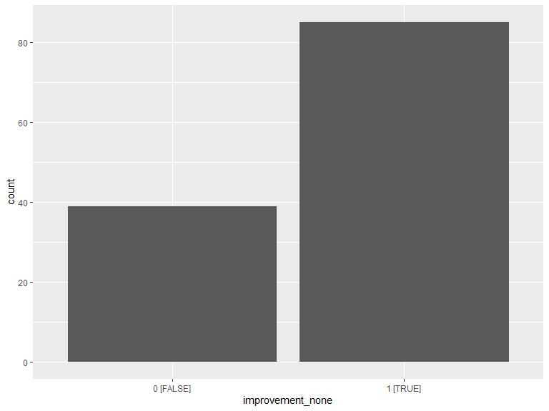

.improv_cnt <- .improv %>%
  group_by(improvement_none) %>%
  dplyr::count() %>%
  arrange(improvement_none)
kable(.improv_cnt, caption = "No area of improvement") %>% kable_styling(bootstrap_options = "striped", full_width = T, position = "left")

No area of improvement

improvement_none	n
0 [FALSE]	39
1 [TRUE]	85

# polgon extraction
improv <- poly_geom[poly_geom$area_type == "improvement", ]

# Map
bm + geom_sf(data = improv, inherit.aes = FALSE, fill = alpha("blue", 0.3), color = alpha("blue", 0.5))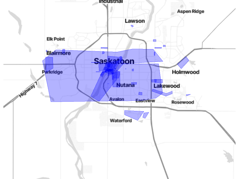

# Min, max, median & mean area of PRN
improv <- improv %>%
  mutate(area_m2 = st_area(.))
kable(t(as.matrix(summary(improv$area_m2))),
  caption = "Area (in square meters) of the perceived improvement areas",
  digits = 1
) %>% kable_styling(bootstrap_options = "striped", full_width = T, position = "left")

Area (in square meters) of the perceived improvement areas

Min.	1st Qu.	Median	Mean	3rd Qu.	Max.
2095.9	62440	154360.2	2227609	526253.1	60269942

2.8.2 Can you locate areas where you have noticed a deterioration of the urban environment?

# extract and recode
.deter <- veritas_main[c("interact_id", "deterioration_none")] %>% dplyr::rename(deterioration_none_code = deterioration_none)
.deter$deterioration_none <- factor(ifelse(.deter$deterioration_none_code == 1, "1 [TRUE]",
  ifelse(.deter$deterioration_none_code == 0, "0 [FALSE]", "N/A")
))

# histogram of answers
ggplot(data = .deter) +
  geom_histogram(aes(x = deterioration_none), stat = "count") +
  scale_x_discrete(labels = function(lbl) str_wrap(lbl, width = 20)) +
  labs(x = "deterioration_none")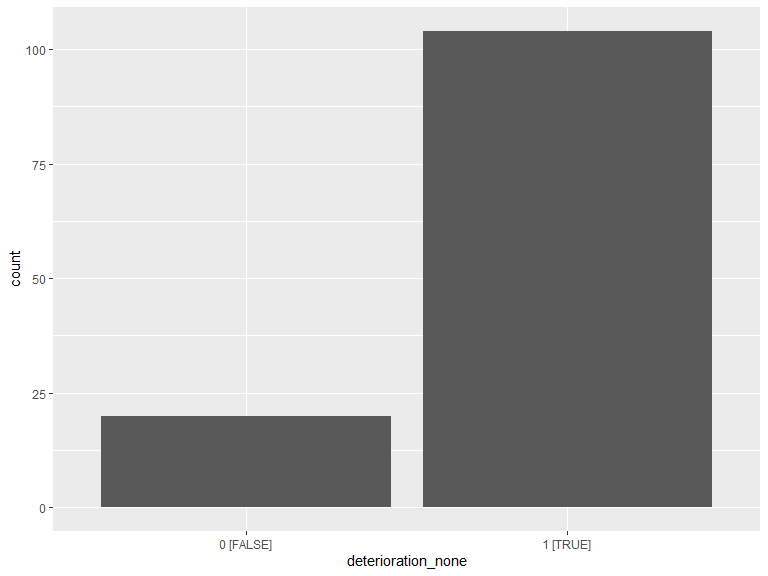

.deter_cnt <- .deter %>%
  group_by(deterioration_none) %>%
  dplyr::count() %>%
  arrange(deterioration_none)
kable(.deter_cnt, caption = "No area of deterioration") %>% kable_styling(bootstrap_options = "striped", full_width = T, position = "left")

No area of deterioration

deterioration_none	n
0 [FALSE]	20
1 [TRUE]	104

# polgon extraction
deter <- poly_geom[poly_geom$area_type == "deterioration", ]

# Map
bm + geom_sf(data = deter, inherit.aes = FALSE, fill = alpha("blue", 0.3), color = alpha("blue", 0.5))

# Min, max, median & mean area of PRN
deter <- deter %>%
  mutate(area_m2 = st_area(.))
kable(t(as.matrix(summary(deter$area_m2))),
  caption = "Area (in square meters) of the perceived deterioration areas",
  digits = 1
) %>%
  kable_styling(bootstrap_options = "striped", full_width = T, position = "left")

Area (in square meters) of the perceived deterioration areas

Min.	1st Qu.	Median	Mean	3rd Qu.	Max.
2885.9	46555.9	142753.1	962796.2	491679.5	11126015

2.9 Section 9: Social contact

2.9.1 Do you visit anyone at his or her home at least once per month?

# extract and recode
.visiting <- veritas_main[c("interact_id", "visiting")] %>% dplyr::rename(visiting_code = visiting)
.visiting$visiting <- factor(ifelse(.visiting$visiting_code == 1, "1 [Yes]",
  ifelse(.visiting$visiting_code == 2, "2 [No]", "N/A")
))

# histogram of answers
ggplot(data = .visiting) +
  geom_histogram(aes(x = visiting), stat = "count") +
  scale_x_discrete(labels = function(lbl) str_wrap(lbl, width = 20)) +
  labs(x = "visiting")

.visiting_cnt <- .visiting %>%
  group_by(visiting) %>%
  dplyr::count() %>%
  arrange(visiting)
kable(.visiting_cnt, caption = "Social contact") %>% kable_styling(bootstrap_options = "striped", full_width = T, position = "left")

Social contact

visiting	n
1 [Yes]	58
2 [No]	66

2.9.2 Great, we are almost done completing this questionnaire. You have documented all your activity places on a map, and specified with whom you generally do these activities. These last few questions concern the people you documented earlier.

# compute statistics on groups / participant
# > one needs to account for participants who did not report any group
.gr_iid_cnt <- as.data.frame(group[c("interact_id")]) %>%
  group_by(interact_id) %>%
  dplyr::count()

# (cont'd) find iid combination without match in veritas group
.no_gr_iid <- anti_join(veritas_main[c("interact_id")], .gr_iid_cnt, by = "interact_id") %>%
  mutate(n = 0)
.gr_iid_cnt <- bind_rows(.gr_iid_cnt, .no_gr_iid)

kable(t(as.matrix(summary(.gr_iid_cnt$n))),
  caption = "Number of groups per participant",
  digits = 1
) %>%
  kable_styling(bootstrap_options = "striped", full_width = T, position = "left")

Number of groups per participant

Min.	1st Qu.	Median	Mean	3rd Qu.	Max.
0	0	0	0.6	1	7

# compute statistics on people / participant
# > one needs to account for participants who did not report any group
.pl_iid_cnt <- as.data.frame(people[c("interact_id")]) %>%
  group_by(interact_id) %>%
  dplyr::count()

# (cont'd) find iid combination without match in veritas group
.no_pl_iid <- anti_join(veritas_main[c("interact_id")], .pl_iid_cnt, by = "interact_id") %>%
  mutate(n = 0)
.pl_iid_cnt <- bind_rows(.pl_iid_cnt, .no_pl_iid)

kable(t(as.matrix(summary(.pl_iid_cnt$n))),
  caption = "Number of people per participant",
  digits = 1
) %>%
  kable_styling(bootstrap_options = "striped", full_width = T, position = "left")

Number of people per participant

Min.	1st Qu.	Median	Mean	3rd Qu.	Max.
0	1	1	2.2	3	13

# histogram
.sc_iid_cnt <- .pl_iid_cnt %>% mutate(soc_type = "people")
.sc_iid_cnt <- .gr_iid_cnt %>%
  mutate(soc_type = "group") %>%
  bind_rows(.sc_iid_cnt)

ggplot(data = .sc_iid_cnt) +
  geom_histogram(aes(x = n, y = stat(count), fill = soc_type), position = "dodge") +
  labs(x = "Social network size by element type", fill = element_blank())

2.9.2.1 Among these people, who do you discuss important matters with?

# extract number of important people / participant
.n_important <- important %>% dplyr::count(interact_id)
.n_people <- people %>% dplyr::count(interact_id)

.n_people_imp <- left_join(veritas_main[c("interact_id")], .n_people, by = "interact_id") %>%
  left_join(.n_important, by = "interact_id") %>%
  mutate_all(~ replace(., is.na(.), 0)) %>%
  dplyr::rename(n_people = n.x, n_important = n.y) %>%
  mutate(pct = 100 * n_important / n_people)

kable(t(as.matrix(summary(.n_people_imp$n_important))),
  caption = "Number of important people per participant",
  digits = 1
) %>%
  kable_styling(bootstrap_options = "striped", full_width = T, position = "left")

Number of important people per participant

Min.	1st Qu.	Median	Mean	3rd Qu.	Max.
0	0	1	1.4	2	10

kable(t(as.matrix(summary(.n_people_imp$pct))),
  caption = "% of important people among social contact per participant",
  digits = 1
) %>%
  kable_styling(bootstrap_options = "striped", full_width = T, position = "left")

% of important people among social contact per participant

Min.	1st Qu.	Median	Mean	3rd Qu.	Max.	NA’s
0	50	100	71.4	100	100	28

2.9.2.2 Among these people, who do you like to socialize with?

# extract number of important people / participant
.n_socialize <- socialize %>% dplyr::count(interact_id)
.n_people <- people %>% dplyr::count(interact_id)

.n_people_soc <- left_join(veritas_main[c("interact_id")], .n_people, by = "interact_id") %>%
  left_join(.n_socialize, by = "interact_id") %>%
  mutate_all(~ replace(., is.na(.), 0)) %>%
  dplyr::rename(n_people = n.x, n_socialize = n.y) %>%
  mutate(pct = 100 * n_socialize / n_people)

kable(t(as.matrix(summary(.n_people_soc$n_socialize))),
  caption = "Number of people with whom to socialize per participant",
  digits = 1
) %>%
  kable_styling(bootstrap_options = "striped", full_width = T, position = "left")

Number of people with whom to socialize per participant

Min.	1st Qu.	Median	Mean	3rd Qu.	Max.
0	0	1	1.8	3	11

kable(t(as.matrix(summary(.n_people_soc$pct))),
  caption = "% of people with whom to  socialize among social contact per participant",
  digits = 1
) %>%
  kable_styling(bootstrap_options = "striped", full_width = T, position = "left")

% of people with whom to socialize among social contact per participant

Min.	1st Qu.	Median	Mean	3rd Qu.	Max.	NA’s
0	84.3	100	85.7	100	100	28

2.9.2.3 Among these people, who do you meet often with but do not necessarily feel close to?

# extract number of important people / participant
.n_not_close <- not_close %>% dplyr::count(interact_id)
.n_people <- people %>% dplyr::count(interact_id)

.n_people_not_close <- left_join(veritas_main[c("interact_id")], .n_people, by = "interact_id") %>%
  left_join(.n_not_close, by = "interact_id") %>%
  mutate_all(~ replace(., is.na(.), 0)) %>%
  dplyr::rename(n_people = n.x, n_not_close = n.y) %>%
  mutate(pct = 100 * n_not_close / n_people)

kable(t(as.matrix(summary(.n_people_not_close$n_not_close))),
  caption = "Number of not so close people per participant",
  digits = 1
) %>%
  kable_styling(bootstrap_options = "striped", full_width = T, position = "left")

Number of not so close people per participant

Min.	1st Qu.	Median	Mean	3rd Qu.	Max.
0	0	0	0.3	0	5

kable(t(as.matrix(summary(.n_people_not_close$pct))),
  caption = "% of not so close people among social contact per participant",
  digits = 1
) %>%
  kable_styling(bootstrap_options = "striped", full_width = T, position = "left")

% of not so close people among social contact per participant

Min.	1st Qu.	Median	Mean	3rd Qu.	Max.	NA’s
0	0	0	12.8	14.9	100	28

2.9.2.4 Among these people, who knows whom?

# extract number of who knows who relationships
.n_relat <- relationship %>%
  filter(relationship_type == 1) %>%
  dplyr::count(interact_id)
.n_people <- people %>% dplyr::count(interact_id)

.n_people_relat <- left_join(veritas_main[c("interact_id")], .n_people, by = "interact_id") %>%
  left_join(.n_relat, by = "interact_id") %>%
  mutate_all(~ replace(., is.na(.), 0)) %>%
  dplyr::rename(n_people = n.x, n_relat = n.y) %>%
  mutate(pct = 100 * n_relat * 2 / (n_people * (n_people - 1))) # potential number of relationships = N x (N -1) / 2

kable(t(as.matrix(summary(.n_people_relat$n_relat))),
  caption = "Number of relationships « who knows who » per participant",
  digits = 1
) %>%
  kable_styling(bootstrap_options = "striped", full_width = T, position = "left")

Number of relationships « who knows who » per participant

Min.	1st Qu.	Median	Mean	3rd Qu.	Max.
0	0	0	3	3	46

kable(t(as.matrix(summary(.n_people_relat$pct))),
  caption = "% of relationships « who knows who » per participant",
  digits = 1
) %>%
  kable_styling(bootstrap_options = "striped", full_width = T, position = "left")

% of relationships « who knows who » per participant

Min.	1st Qu.	Median	Mean	3rd Qu.	Max.	NA’s
0	59.2	96.7	73.7	100	100	70

2.10 Derived metrics

2.10.1 Existence of improvement and deterioration areas by participant

Combination of improvement and/or deterioration areas per participant

# cross tab of improvement vs deteriation areas
.improv <- improv[c("interact_id")] %>%
  mutate(improv = "Improvement")
.deter <- deter[c("interact_id")] %>%
  mutate(deter = "Deterioration")
.ct_impr_deter <- veritas_main[c("interact_id")] %>%
  transmute(interact_id = as.character(interact_id)) %>%
  left_join(.improv, by = "interact_id") %>%
  left_join(.deter, by = "interact_id") %>%
  mutate_all(~ replace(., is.na(.), "N/A"))

kable(table(.ct_impr_deter$improv, .ct_impr_deter$deter), caption = "Improvement vs. deterioration") %>%
  kable_styling(bootstrap_options = "striped", full_width = T, position = "left", row_label_position = "r") %>%
  column_spec(1, bold = T)

Improvement vs. deterioration

	Deterioration	N/A
Improvement	14	21
N/A	5	84

2.10.2 Transportation mode preferences

Based on the answers to the question Usually, how do you go there? (Check all that apply.).

# code  en
# 1 By car and you drive
# 2 By car and someone else drives
# 3 By taxi/Uber
# 4 On foot
# 5 By bike
# 6 By bus
# 7 By subway
# 8 By train
# 99    Other

loc_labels <- data.frame(location_category = c(2:26), description = c(
  " 2 [Other residence]",
  " 3 [Work]",
  " 4 [School/College/University]",
  " 5 [Supermarket]",
  " 6 [Public/farmer’s market]",
  " 7 [Bakery]",
  " 8 [Specialty food store]",
  " 9 [Convenience store/Dépanneur]",
  "10 [Liquor store/SAQ]",
  "11 [Bank]",
  "12 [Hair salon/barbershop]",
  "13 [Post office]",
  "14 [Drugstore]",
  "15 [Doctor/healthcare provider]",
  "16 [Public transit stop]",
  "17 [Leisure-time physical activity]",
  "18 [Park]",
  "19 [Cultural activity]",
  "20 [Volunteering place]",
  "21 [Religious/spiritual activity]",
  "22 [Restaurant, café, bar, etc.]",
  "23 [Take-out]",
  "24 [Walk]",
  "25 [Other place]",
  "26 [Social contact residence]"
))

# extract and summary stats
.tm <- locations %>%
  st_set_geometry(NULL) %>%
  filter(location_category != 1) %>%
  left_join(loc_labels)

.tm_grouped <- .tm %>%
  group_by(description) %>%
  dplyr::summarise(
    N = n(), "By car (driver)" = sum(location_tmode_1),
    "By car (passenger)" = sum(location_tmode_2),
    "By taxi/Uber" = sum(location_tmode_3),
    "On foot" = sum(location_tmode_4),
    "By bike" = sum(location_tmode_5),
    "By bus" = sum(location_tmode_6),
    "By train" = sum(location_tmode_7),
    "Other" = sum(location_tmode_99)
  )

kable(.tm_grouped, caption = "Transportation mode preferences") %>% kable_styling(bootstrap_options = "striped", full_width = T, position = "left")

Transportation mode preferences

description	N	By car (driver)	By car (passenger)	By taxi/Uber	On foot	By bike	By bus	By train	Other
2 [Other residence]	19	7	8	0	3	1	7	0	1
3 [Work]	94	36	10	4	22	8	23	0	22
4 [School/College/University]	48	9	5	0	16	1	11	0	20
5 [Supermarket]	265	155	46	0	77	10	40	0	2
6 [Public/farmer’s market]	11	8	2	0	2	1	2	0	0
7 [Bakery]	37	15	7	0	19	1	2	0	0
8 [Specialty food store]	54	29	8	1	24	1	4	0	0
9 [Convenience store/Dépanneur]	66	16	7	0	45	2	9	0	1
10 [Liquor store/SAQ]	76	46	11	0	23	1	6	0	0
11 [Bank]	98	51	5	1	38	4	17	0	1
12 [Hair salon/barbershop]	59	37	5	1	14	5	11	0	0
13 [Post office]	56	25	1	0	31	3	9	0	1
14 [Drugstore]	90	46	9	0	46	4	14	0	0
15 [Doctor/healthcare provider]	99	56	9	8	14	6	29	0	4
16 [Public transit stop]	108	2	1	1	76	0	37	0	0
17 [Leisure-time physical activity]	76	40	15	0	15	12	2	0	7
18 [Park]	112	30	12	0	74	4	3	0	1
19 [Cultural activity]	1	0	1	0	1	0	0	0	0
20 [Volunteering place]	15	6	1	0	5	0	3	0	4
21 [Religious/spiritual activity]	11	3	1	0	4	0	0	0	3
22 [Restaurant, café, bar, etc.]	123	60	33	5	44	4	17	0	0
23 [Take-out]	151	57	28	1	20	1	10	0	44
24 [Walk]	131	16	3	1	111	3	6	0	4
25 [Other place]	34	23	2	2	5	2	3	0	1

# graph
.tm1 <- .tm %>%
  filter(location_tmode_1 == 1) %>%
  mutate(tm = "[1] By car (driver)")
.tm2 <- .tm %>%
  filter(location_tmode_2 == 1) %>%
  mutate(tm = "[2] By car (passenger)")
.tm3 <- .tm %>%
  filter(location_tmode_3 == 1) %>%
  mutate(tm = "[3] By taxi/Uber")
.tm4 <- .tm %>%
  filter(location_tmode_4 == 1) %>%
  mutate(tm = "[4] On foot")
.tm5 <- .tm %>%
  filter(location_tmode_5 == 1) %>%
  mutate(tm = "[5] By bike")
.tm6 <- .tm %>%
  filter(location_tmode_6 == 1) %>%
  mutate(tm = "[6] By bus")
# .tm7 <- .tm %>%                       # Empty dataframe -> error when creating tm col.
#   filter(location_tmode_7 == 1) %>%
#   mutate(tm = "[7] By train")
.tm99 <- .tm %>%
  filter(location_tmode_99 == 1) %>%
  mutate(tm = "[99] Other")
.tm <- bind_rows(.tm1, .tm2) %>%
  bind_rows(.tm3) %>%
  bind_rows(.tm4) %>%
  bind_rows(.tm5) %>%
  bind_rows(.tm6) %>%
  #  bind_rows(.tm7) %>%
  bind_rows(.tm99)

# histogram of answers
ggplot(data = .tm) +
  geom_bar(aes(x = fct_rev(description), fill = tm), position = "fill") +
  scale_fill_brewer(palette = "Set3", name = "Transport modes") +
  scale_y_continuous(labels = percent) +
  labs(y = "Proportion of transportation mode by location category", x = element_blank()) +
  coord_flip() +
  theme(legend.position = "bottom", legend.justification = c(0, 0), legend.text = element_text(size = 8)) +
  guides(fill = guide_legend(nrow = 3))

2.10.3 Visiting places alone

Based on the answers to the question Do you usually go to this place alone or with other people?.

loc_labels <- data.frame(location_category = c(2:26), description = c(
  " 2 [Other residence]",
  " 3 [Work]",
  " 4 [School/College/University]",
  " 5 [Supermarket]",
  " 6 [Public/farmer’s market]",
  " 7 [Bakery]",
  " 8 [Specialty food store]",
  " 9 [Convenience store/Dépanneur]",
  "10 [Liquor store/SAQ]",
  "11 [Bank]",
  "12 [Hair salon/barbershop]",
  "13 [Post office]",
  "14 [Drugstore]",
  "15 [Doctor/healthcare provider]",
  "16 [Public transit stop]",
  "17 [Leisure-time physical activity]",
  "18 [Park]",
  "19 [Cultural activity]",
  "20 [Volunteering place]",
  "21 [Religious/spiritual activity]",
  "22 [Restaurant, café, bar, etc.]",
  "23 [Take-out]",
  "24 [Walk]",
  "25 [Other place]",
  "26 [Social contact residence]"
))

# extract and summary stats
.alone <- locations %>%
  st_set_geometry(NULL) %>%
  filter(location_category != 1) %>%
  left_join(loc_labels) %>%
  mutate(location_alone_recode = case_when(
    location_alone2 == 1 ~ 1,
    location_alone2 == 2 ~ 0
  ))

.alone_grouped <- .alone %>%
  group_by(description) %>%
  dplyr::summarise(
    N = n(), "Visited alone" = sum(location_alone_recode),
    "Visited alone (%)" = round(sum(location_alone_recode) * 100.0 / n(), digits = 1)
  )

kable(.alone_grouped, caption = "Visiting places alone") %>% kable_styling(bootstrap_options = "striped", full_width = T, position = "left")

Visiting places alone

description	N	Visited alone	Visited alone (%)
2 [Other residence]	19	1	5.3
3 [Work]	94	39	41.5
4 [School/College/University]	48	34	70.8
5 [Supermarket]	265	200	75.5
6 [Public/farmer’s market]	11	7	63.6
7 [Bakery]	37	22	59.5
8 [Specialty food store]	54	36	66.7
9 [Convenience store/Dépanneur]	66	49	74.2
10 [Liquor store/SAQ]	76	51	67.1
11 [Bank]	98	90	91.8
12 [Hair salon/barbershop]	59	56	94.9
13 [Post office]	56	50	89.3
14 [Drugstore]	90	78	86.7
15 [Doctor/healthcare provider]	99	84	84.8
16 [Public transit stop]	108	96	88.9
17 [Leisure-time physical activity]	76	37	48.7
18 [Park]	112	55	49.1
19 [Cultural activity]	1	0	0.0
20 [Volunteering place]	15	8	53.3
21 [Religious/spiritual activity]	11	4	36.4
22 [Restaurant, café, bar, etc.]	123	43	35.0
23 [Take-out]	151	76	50.3
24 [Walk]	131	94	71.8
25 [Other place]	34	20	58.8

# histogram of answers
ggplot(data = .alone) +
  geom_bar(aes(x = fct_rev(description), fill = factor(location_alone2)), position = "fill") +
  scale_fill_brewer(palette = "Set3", name = "Visiting places", labels = c("Alone", "With someone")) +
  scale_y_continuous(labels = percent) +
  labs(y = "Proportion of places visited alone", x = element_blank()) +
  coord_flip()

2.10.4 Visit frequency

Based on the answers to the question How often do you go there?.

loc_labels <- data.frame(location_category = c(2:26), description = c(
  " 2 [Other residence]",
  " 3 [Work]",
  " 4 [School/College/University]",
  " 5 [Supermarket]",
  " 6 [Public/farmer’s market]",
  " 7 [Bakery]",
  " 8 [Specialty food store]",
  " 9 [Convenience store/Dépanneur]",
  "10 [Liquor store/SAQ]",
  "11 [Bank]",
  "12 [Hair salon/barbershop]",
  "13 [Post office]",
  "14 [Drugstore]",
  "15 [Doctor/healthcare provider]",
  "16 [Public transit stop]",
  "17 [Leisure-time physical activity]",
  "18 [Park]",
  "19 [Cultural activity]",
  "20 [Volunteering place]",
  "21 [Religious/spiritual activity]",
  "22 [Restaurant, café, bar, etc.]",
  "23 [Take-out]",
  "24 [Walk]",
  "25 [Other place]",
  "26 [Social contact residence]"
))

# extract and summary stats
.freq <- locations %>%
  st_set_geometry(NULL) %>%
  filter(location_category != 1) %>%
  left_join(loc_labels)

.freq_grouped <- .freq %>%
  group_by(description) %>%
  dplyr::summarise(
    N = n(), min = min(location_freq_visit),
    max = max(location_freq_visit),
    mean = mean(location_freq_visit),
    median = median(location_freq_visit),
    sd = sd(location_freq_visit)
  )

kable(.freq_grouped, caption = "Visit frequency (expressed in times/year)") %>% kable_styling(bootstrap_options = "striped", full_width = T, position = "left")

Visit frequency (expressed in times/year)

description	N	min	max	mean	median	sd
2 [Other residence]	19	1	520	120	104	125.471765
3 [Work]	94	0	5200	289	260	527.252580
4 [School/College/University]	48	0	5200	340	312	730.791700
5 [Supermarket]	265	0	520	44	24	51.185853
6 [Public/farmer’s market]	11	5	104	30	12	36.903560
7 [Bakery]	37	3	104	31	12	30.099410
8 [Specialty food store]	54	1	104	17	12	19.101343
9 [Convenience store/Dépanneur]	66	1	364	63	36	72.367698
10 [Liquor store/SAQ]	76	1	156	20	12	21.986583
11 [Bank]	98	0	104	12	12	15.582146
12 [Hair salon/barbershop]	59	0	312	11	4	40.489661
13 [Post office]	56	0	52	12	6	14.179908
14 [Drugstore]	90	1	260	23	12	35.305870
15 [Doctor/healthcare provider]	99	0	60	5	3	9.094377
16 [Public transit stop]	108	2	520	112	52	123.768743
17 [Leisure-time physical activity]	76	1	5200	172	52	592.713557
18 [Park]	112	1	728	76	48	107.139440
19 [Cultural activity]	1	1	1	1	1	NA
20 [Volunteering place]	15	1	52000	3498	24	13417.481594
21 [Religious/spiritual activity]	11	1	5200	590	52	1536.676420
22 [Restaurant, café, bar, etc.]	123	1	264	26	12	34.766056
23 [Take-out]	151	0	208	22	12	31.706350
24 [Walk]	131	1	884	110	52	143.860672
25 [Other place]	34	1	624	49	12	112.843289

# graph
ggplot(data = .freq) +
  geom_boxplot(aes(x = fct_rev(description), y = location_freq_visit)) +
  scale_y_continuous(limits = c(0, 365)) +
  labs(y = "Visits/year (Frequency over 1 visit/day not shown)", x = element_blank()) +
  coord_flip()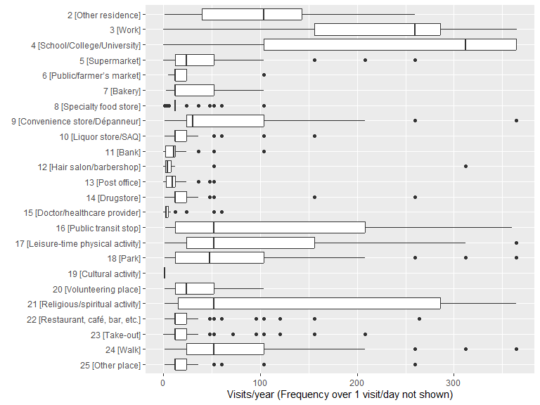

2.10.5 Spatial indicators: Camille Perchoux’s toolbox

Below is a list of indicators proposed by Camille Perchoux in her paper Assessing patterns of spatial behavior in health studies: Their socio-demographic determinants and associations with transportation modes (the RECORD Cohort Study).

-- Reading Camille tbx indics from Essence table
SELECT interact_id,
  n_acti_places, n_weekly_vst, n_acti_types,
  cvx_perimeter, cvx_surface,
  min_length, max_length, median_length, 
  pct_visits_neighb, 
  n_acti_prn, pct_visits_prn, prn_area_km2
FROM essence_table.essence_perchoux_tbx
WHERE city_id = 'Saskatoon' AND wave_id = 2 AND status = 'new'

2.10.5.1 Indicators related to the lifestyle

Indicators	Measurement approach
Number of activity places (n_acti_places)	Count of activity places
Number of visits to places per week (n_weekly_vst)	Number of activity places per individual multiplied by the frequency of visit per week to each location, excluding the residence
Number of activity types (n_acti_types)	6 types of activities considered: 1-Residential; 2-Occupation; 3-Shopping activities; 4-Services; 5-Transportation; 6-Leisure activities (NB original categories were as follow: 1-Residential; 2-work; 3-food and other services; 4-transport station/stop; 5-recreational activity; 6-social activity)

LLindic <- ess.tab.camille %>%
  select("interact_id", "n_acti_places", "n_weekly_vst", "n_acti_types")
.llmtx <- as.matrix(summary(LLindic[c("n_acti_places", "n_weekly_vst", "n_acti_types")], digits = 1))
.llmtx <- apply(.llmtx, 1:2, function(x) strsplit(as.character(x), ":")[[1]][2])
rownames(.llmtx) <- c("Min.   ", "1st Qu.", "Median ", "Mean   ", "3rd Qu.", "Max.   ")
kable(.llmtx, caption = "Lifestyle statistics") %>% kable_styling(bootstrap_options = "striped", full_width = T, position = "left")

Lifestyle statistics

	n_acti_places	n_weekly_vst	n_acti_types
Min.	2	1	2
1st Qu.	10	11	5
Median	14	17	5
Mean	16	29	5
3rd Qu.	21	24	6
Max.	37	1008	6

2.10.5.2 Indicators related to the geometry of the activity space

Indicators	Measurement approach
Perimeter of the convex hull (cvx_perimeter)	Perimeter of the smallest polygon containing all the activity locations of the participant (unit: km)
Surface of the convex hull (cvx_surface)	Surface of the smallest polygon containing all the activity locations of the participant (unit: km2)
Minimal road network distance from the residence to an activity place (min_length)	Minimal distance from the residence to an activity place using the road network (in meters)
Maximal road network distance from the residence to an activity place (max_length)	Maximal distance from the residence to an activity place using the road network (in meters)
Median road network distance from the residence to all activity places (median_length)	Median distance from home to all activity places using the road network (in meters)

ASindic <- ess.tab.camille %>%
  select("interact_id", "cvx_perimeter", "cvx_surface", "min_length", "max_length", "median_length")
.asmtx <- as.matrix(summary(ASindic[c("cvx_perimeter", "cvx_surface", "min_length", "max_length", "median_length")], digits = 1))
.asmtx <- apply(.asmtx, 1:2, function(x) strsplit(as.character(x), ":")[[1]][2])
rownames(.asmtx) <- c("Min.   ", "1st Qu.", "Median ", "Mean   ", "3rd Qu.", "Max.   ")
.asmtx[is.na(.asmtx)] <- 0
kable(.asmtx, caption = "Activity space statistics") %>% kable_styling(bootstrap_options = "striped", full_width = T, position = "left")

Activity space statistics

	cvx_perimeter	cvx_surface	min_length	max_length	median_length
Min.	1e-02	0	2e-01	3e+01	3e+01
1st Qu.	1e+01	7	1e+01	6e+03	1e+03
Median	2e+01	20	1e+02	8e+03	2e+03
Mean	7e+01	82	4e+02	1e+04	4e+03
3rd Qu.	3e+01	34	4e+02	1e+04	3e+03
Max.	5e+03	4768	5e+03	1e+05	1e+05

2.10.5.3 Indicators related to the importance of the residential neighborhood

Indicators	Measurement approach
Percentage of visits to places in the residential neighborhood (pct_visits_neighb)	Count of visits to places within the 500 m road network buffer centered on the residence divided by the total number of visits to places
Number of activity locations in the PRN (n_acti_prn)	Count of activity locations in the PRN
Percentage of visits in the PRN (pct_visits_prn)	Count of visits to places in the PRN divided by the total number of visits to places
Surface of the PRN (prn_area_km2)	Unit: km2

RNindic <- ess.tab.camille %>%
  select("interact_id", "pct_visits_neighb", "n_acti_prn", "pct_visits_prn", "prn_area_km2")
RNindic <- RNindic[RNindic$interact_id %in% prn$interact_id, ]
.rnmtx <- as.matrix(summary(RNindic[c("pct_visits_neighb", "n_acti_prn", "pct_visits_prn", "prn_area_km2")], digits = 1))
.rnmtx <- apply(.rnmtx, 1:2, function(x) strsplit(as.character(x), ":")[[1]][2])
rownames(.rnmtx) <- c("Min.   ", "1st Qu.", "Median ", "Mean   ", "3rd Qu.", "Max.   ", "N/A.")
.rnmtx[is.na(.rnmtx)] <- 0
kable(.rnmtx, caption = "Residential neighbourhood statistics") %>% kable_styling(bootstrap_options = "striped", full_width = T, position = "left")

Residential neighbourhood statistics

	pct_visits_neighb	n_acti_prn	pct_visits_prn	prn_area_km2
Min.	0	0	0	0.005
1st Qu.	4	1	8	0.273
Median	27	3	41	0.742
Mean	30	3	42	1.050
3rd Qu.	45	5	71	1.433
Max.	93	16	100	6.363
N/A.	63	0	0	0

Only participants with valid PRN considered in Residential Neighbourhood indicators (= 110 participants).

2.10.6 Social indicators: Alexandre Naud’s toolbox

See Alex’s document for a more comprehensive presentation of the social indicators.

-- Reading Alex tbx indics from Essence table
SELECT interact_id,
  people_degree, 
  socialize_size, socialize_meet, socialize_chat,
  important_size, group_degree, simmelian
FROM essence_table.essence_naud_social
WHERE city_id = 'Saskatoon' AND wave_id = 2 AND status = 'new'

2.10.6.1 Number of people in the network (people_degree)

ggplot(ess.tab.alex) +
  geom_histogram(aes(x = people_degree))

kable(t(as.matrix(summary(ess.tab.alex$people_degree))), caption = "people_degree") %>% kable_styling(bootstrap_options = "striped", full_width = T, position = "left")

people_degree

Min.	1st Qu.	Median	Mean	3rd Qu.	Max.
0	1	1	2.217742	3	13

2.10.6.2 Simmelian Brokerage (simmelian)

ggplot(ess.tab.alex) +
  geom_histogram(aes(x = simmelian))

kable(t(as.matrix(summary(ess.tab.alex$simmelian))), caption = "simmelian") %>% kable_styling(bootstrap_options = "striped", full_width = T, position = "left")

simmelian

Min.	1st Qu.	Median	Mean	3rd Qu.	Max.	NA’s
1	1.744048	2.6	5.1199	4.75	74.67677	50

2.10.6.3 Number of people with whom the participant like to socialize (socialize_size)

ggplot(ess.tab.alex) +
  geom_histogram(aes(x = socialize_size))

kable(t(as.matrix(summary(ess.tab.alex$socialize_size))), caption = "socialize_size") %>% kable_styling(bootstrap_options = "striped", full_width = T, position = "left")

socialize_size

Min.	1st Qu.	Median	Mean	3rd Qu.	Max.
0	0	1	1.83871	3	11

2.10.6.4 Weekly face-to-face interactions among people with whom the participant like to socialize (socialize_meet)

ggplot(filter(ess.tab.alex, socialize_meet < 100)) +
  geom_histogram(aes(x = socialize_meet)) +
  annotate(geom = "text", x = 75, y = 100, label = "X-axis: values over 100 not displayed", alpha = .5)

kable(t(as.matrix(summary(ess.tab.alex$socialize_meet))), caption = "socialize_meet") %>% kable_styling(bootstrap_options = "striped", full_width = T, position = "left")

socialize_meet

Min.	1st Qu.	Median	Mean	3rd Qu.	Max.
0	0	302	446.7097	423.5	5457

2.10.6.5 Weekly ICT interactions among people with whom the participant like to socialize (socialize_chat)

ggplot(filter(ess.tab.alex, socialize_chat < 100)) +
  geom_histogram(aes(x = socialize_chat)) +
  annotate(geom = "text", x = 55, y = 100, label = "X-axis: values over 100 not displayed", alpha = .5)

kable(t(as.matrix(summary(ess.tab.alex$socialize_chat))), caption = "socialize_chat") %>% kable_styling(bootstrap_options = "striped", full_width = T, position = "left")

socialize_chat

Min.	1st Qu.	Median	Mean	3rd Qu.	Max.
0	0	364	1021.798	734	15600

2.10.6.6 Number of people with whom the participant discuss important matters (important_size)

ggplot(ess.tab.alex) +
  geom_histogram(aes(x = important_size))

kable(t(as.matrix(summary(ess.tab.alex$important_size))), caption = "important_size") %>% kable_styling(bootstrap_options = "striped", full_width = T, position = "left")

important_size

Min.	1st Qu.	Median	Mean	3rd Qu.	Max.
0	0	1	1.395161	2	10

2.10.6.7 Number of people in all groups (group_degree)

ggplot(filter(ess.tab.alex, group_degree < 100)) +
  geom_histogram(aes(x = group_degree)) +
  annotate(geom = "text", x = 20, y = 100, label = "X-axis: values over 100 not displayed", alpha = .5)

kable(t(as.matrix(summary(ess.tab.alex$group_degree))), caption = "group_degree") %>% kable_styling(bootstrap_options = "striped", full_width = T, position = "left")

group_degree

Min.	1st Qu.	Median	Mean	3rd Qu.	Max.
0	0	0	3.145161	3.25	92

3 Basic descriptive statistics for returning participants

3.1 Section 1: Residence and Neighbourhood

3.1.1 Now, let’s start with your home. What is your address?

home_location <- locations[locations$location_category == 1, ]

## version ggmap
skt_aoi <- st_bbox(home_location)
names(skt_aoi) <- c("left", "bottom", "right", "top")
skt_aoi[["left"]] <- skt_aoi[["left"]] - .07
skt_aoi[["right"]] <- skt_aoi[["right"]] + .07
skt_aoi[["top"]] <- skt_aoi[["top"]] + .01
skt_aoi[["bottom"]] <- skt_aoi[["bottom"]] - .01

bm <- get_stadiamap(skt_aoi, zoom = 11, maptype = "stamen_toner_lite") %>%
  ggmap(extent = "device")
bm + geom_sf(data = st_jitter(home_location, .008), inherit.aes = FALSE, color = "blue", size = 1.8, alpha = .3) # see https://github.com/r-spatial/sf/issues/336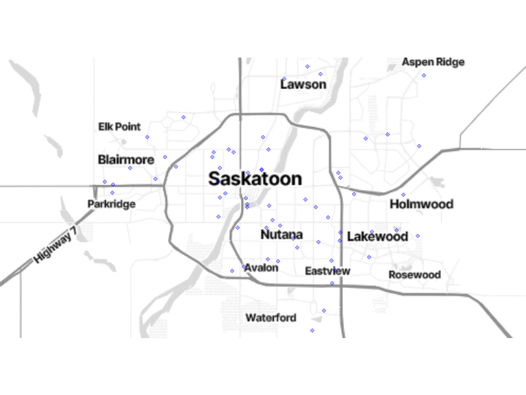

NB: Home locations have been randomly shifted from their original position to protect privacy.

# Number of participants by municipalites
home_by_municipalites <- st_join(home_location, municipalities["NAME"])
home_by_mun_cnt <- as.data.frame(home_by_municipalites) %>%
  group_by(NAME) %>%
  dplyr::count() %>%
  arrange(desc(n), NAME)
home_by_mun_cnt$Shape <- NULL
kable(home_by_mun_cnt, caption = "Number of participants by municipalities") %>% kable_styling(bootstrap_options = "striped", full_width = T, position = "left")

Number of participants by municipalities

NAME	n
Saskatoon	63

3.1.2 If you were asked to draw the boundaries of your neighbourhood, what would they be?

prn <- poly_geom[poly_geom$area_type == "neighborhood", ]

## version ggmap
bm + geom_sf(data = prn, inherit.aes = FALSE, fill = alpha("blue", 0.05), color = alpha("blue", 0.3))

# Min, max, median & mean area of PRN
prn$area_m2 <- st_area(prn$geom)
kable(t(as.matrix(summary(prn$area_m2))),
  caption = "Area (in square meters) of the perceived residential neighborhood",
  digits = 1
) %>%
  kable_styling(bootstrap_options = "striped", full_width = T, position = "left")

Area (in square meters) of the perceived residential neighborhood

Min.	1st Qu.	Median	Mean	3rd Qu.	Max.
7007.5	588305.4	1092275	1400642	1948467	5287563

NB only 60 valid neighborhoods were collected, as many participants struggled to draw polygons on the map.

3.1.3 How attached are you to your neighbourhood?

# extract and recode
.ngh_att <- veritas_main[veritas_main$neighbourhood_attach != 99, c("interact_id", "neighbourhood_attach")] %>% dplyr::rename(neighbourhood_attach_code = neighbourhood_attach)
.ngh_att$neighbourhood_attach <- factor(ifelse(.ngh_att$neighbourhood_attach_code == 1, "1 [Not attached at all]",
  ifelse(.ngh_att$neighbourhood_attach_code == 6, "6 [Very attached]",
    .ngh_att$neighbourhood_attach_code
  )
))

# histogram of attachment
ggplot(data = .ngh_att) +
  geom_histogram(aes(x = neighbourhood_attach), stat = "count") +
  scale_x_discrete(labels = function(lbl) str_wrap(lbl, width = 20)) +
  labs(x = "neighbourhood_attach")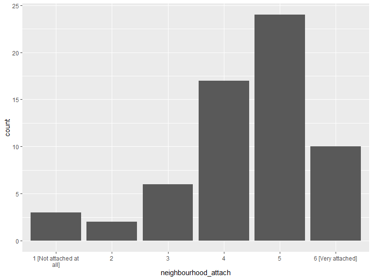

.ngh_att_cnt <- .ngh_att %>%
  group_by(neighbourhood_attach) %>%
  dplyr::count() %>%
  arrange(neighbourhood_attach)
kable(.ngh_att_cnt, caption = "Neigbourhood attachment") %>% 
  kable_styling(bootstrap_options = "striped", full_width = T, position = "left")

Neigbourhood attachment

neighbourhood_attach	n
1 [Not attached at all]	3
2	2
3	6
4	17
5	24
6 [Very attached]	10

3.1.4 On average, how many hours per day do you spend outside of your home?

# histogram of n hours out
ggplot(data = veritas_main) +
  geom_histogram(aes(x = hours_out))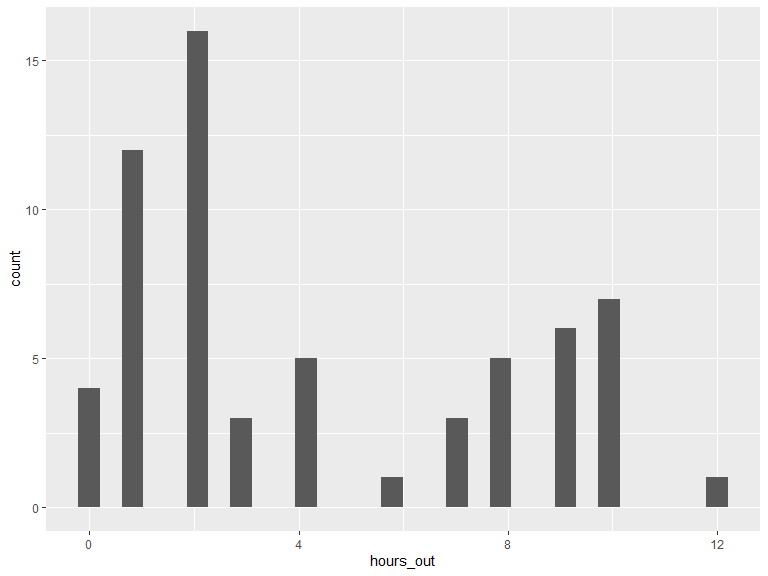

# Min, max, median & mean hours/day out
kable(t(as.matrix(summary(veritas_main$hours_out))),
  caption = "Hours/day outside home",
  digits = 1
) %>%
  kable_styling(bootstrap_options = "striped", full_width = T, position = "left")

Hours/day outside home

Min.	1st Qu.	Median	Mean	3rd Qu.	Max.
0	1.5	2	4.4	8	12

3.1.5 Of this time spent outside your home, on average how many hours do you spend outside your neighbourhood?

# histogram of n hours out
ggplot(data = veritas_main) +
  geom_histogram(aes(x = hours_out_neighb))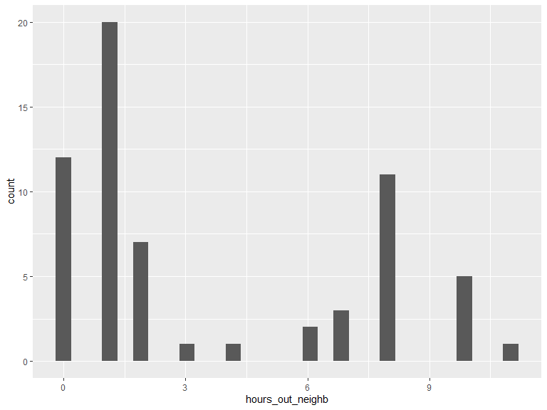

# Min, max, median & mean hours/day out of neighborhood
kable(t(as.matrix(summary(veritas_main$hours_out_neighb))),
  caption = "Hours/day outside neighbourhood",
  digits = 1
) %>%
  kable_styling(bootstrap_options = "striped", full_width = T, position = "left")

Hours/day outside neighbourhood

Min.	1st Qu.	Median	Mean	3rd Qu.	Max.
0	1	1	3.5	8	11

3.1.6 Are there one or more areas close to where you live that you tend to avoid because you do not feel safe there (for any reason)?

# extract and recode
.unsafe <- veritas_main[c("interact_id", "unsafe_area")] %>% dplyr::rename(unsafe_area_code = unsafe_area)
.unsafe$unsafe_area <- factor(ifelse(.unsafe$unsafe_area_code == 1, "1 [Yes]",
  ifelse(.unsafe$unsafe_area_code == 2, "2 [No]", "N/A")
))

# histogram of answers
ggplot(data = .unsafe) +
  geom_histogram(aes(x = unsafe_area), stat = "count") +
  scale_x_discrete(labels = function(lbl) str_wrap(lbl, width = 20)) +
  labs(x = "unsafe_area")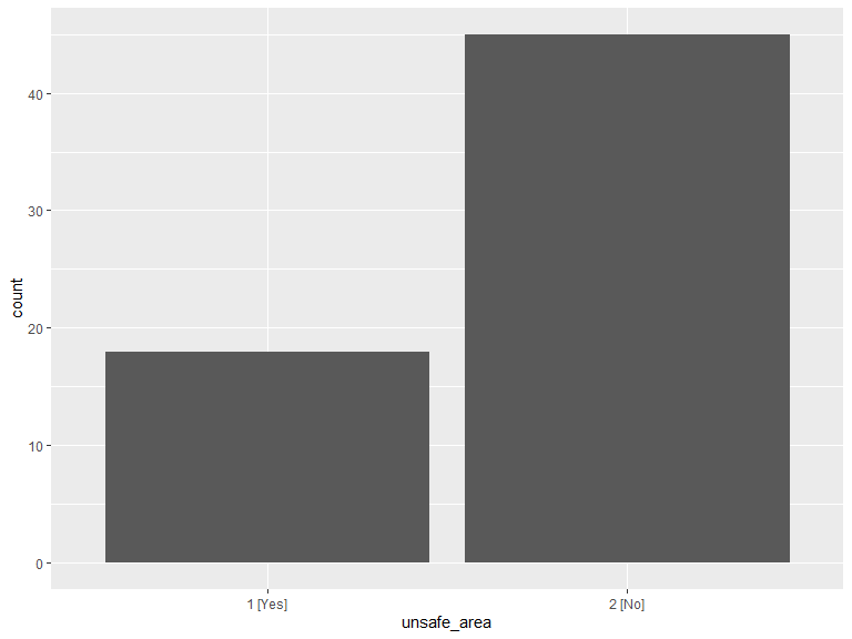

.unsafe_cnt <- .unsafe %>%
  group_by(unsafe_area) %>%
  dplyr::count() %>%
  arrange(unsafe_area)
kable(.unsafe_cnt, caption = "Unsafe areas") %>% 
  kable_styling(bootstrap_options = "striped", full_width = T, position = "left")

Unsafe areas

unsafe_area	n
1 [Yes]	18
2 [No]	45

# map
unsafe <- poly_geom[poly_geom$area_type == "unsafe area", ]

## version ggmap
bm + geom_sf(data = unsafe, inherit.aes = FALSE, fill = alpha("blue", 0.3), color = alpha("blue", 0.5))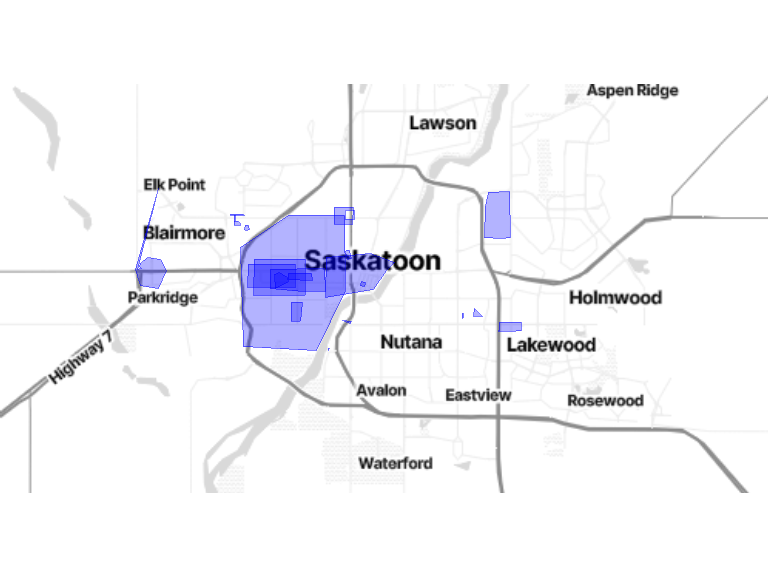

# Min, max, median & mean area of PRN
unsafe$area_m2 <- st_area(unsafe$geom)
kable(t(as.matrix(summary(unsafe$area_m2))),
  caption = "Area (in square meters) of the perceived unsafe area",
  digits = 1
) %>%
  kable_styling(bootstrap_options = "striped", full_width = T, position = "left")

Area (in square meters) of the perceived unsafe area

Min.	1st Qu.	Median	Mean	3rd Qu.	Max.
1301.4	42224.1	181229.3	1106828	1032925	11301512

3.1.7 Do you spend the night somewhere other than your home at least once per week?

# extract and recode
.o_res <- veritas_main[c("interact_id", "other_resid")] %>% dplyr::rename(other_resid_code = other_resid)
.o_res$other_resid <- factor(ifelse(.o_res$other_resid_code == 1, "1 [Yes]",
  ifelse(.o_res$other_resid_code == 2, "2 [No]", "N/A")
))

# histogram of answers
ggplot(data = .o_res) +
  geom_histogram(aes(x = other_resid), stat = "count") +
  scale_x_discrete(labels = function(lbl) str_wrap(lbl, width = 20)) +
  labs(x = "other_resid")

.o_res_cnt <- .o_res %>%
  group_by(other_resid) %>%
  dplyr::count() %>%
  arrange(other_resid)
kable(.o_res_cnt, caption = "Other residence") %>% 
  kable_styling(bootstrap_options = "striped", full_width = T, position = "left")

Other residence

other_resid	n
1 [Yes]	5
2 [No]	58

3.2 Section 2: Occupation

3.2.1 Are you currently working?

# extract and recode
.work <- veritas_main[c("interact_id", "working")] %>% dplyr::rename(working_code = working)
.work$working <- factor(ifelse(.work$working_code == 1, "1 [Yes]",
  ifelse(.work$working_code == 2, "2 [No]", "N/A")
))

# histogram of answers
ggplot(data = .work) +
  geom_histogram(aes(x = working), stat = "count") +
  scale_x_discrete(labels = function(lbl) str_wrap(lbl, width = 20)) +
  labs(x = "working")

.work_cnt <- .work %>%
  group_by(working) %>%
  dplyr::count() %>%
  arrange(working)
kable(.work_cnt, caption = "Currently working") %>% 
  kable_styling(bootstrap_options = "striped", full_width = T, position = "left")

Currently working

working	n
1 [Yes]	45
2 [No]	18

3.2.2 Where do you work?

work_location <- locations[locations$location_category == 3, ]

bm + geom_sf(data = work_location, inherit.aes = FALSE, color = "blue", size = 1.8, alpha = .3)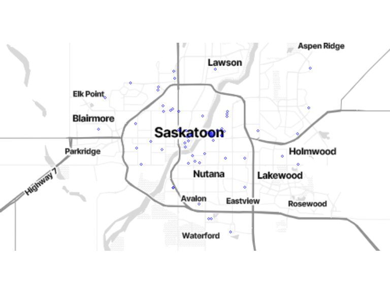

3.2.3 On average, how many hours per week do you work?

# histogram of n hours out
ggplot(data = veritas_main[veritas_main$working == 1, ]) +
  geom_histogram(aes(x = work_hours))

# Min, max, median & mean hours/day out
kable(t(as.matrix(summary(veritas_main$work_hours[veritas_main$working == 1]))),
  caption = "Work hours/week",
  digits = 1
) %>%
  kable_styling(bootstrap_options = "striped", full_width = T, position = "left")

Work hours/week

Min.	1st Qu.	Median	Mean	3rd Qu.	Max.
0	35	38	37.3	40	60

3.2.4 Are you currently a registered student?

# extract and recode
.study <- veritas_main[c("interact_id", "studying")] %>% dplyr::rename(studying_code = studying)
.study$studying <- factor(ifelse(.study$studying_code == 1, "1 [Yes]",
  ifelse(.study$studying_code == 2, "2 [No]", "N/A")
))

# histogram of answers
ggplot(data = .study) +
  geom_histogram(aes(x = studying), stat = "count") +
  scale_x_discrete(labels = function(lbl) str_wrap(lbl, width = 20)) +
  labs(x = "Studying")

.study_cnt <- .study %>%
  group_by(studying) %>%
  dplyr::count() %>%
  arrange(studying)
kable(.study_cnt, caption = "Currently studying") %>% kable_styling(bootstrap_options = "striped", full_width = T, position = "left")

Currently studying

studying	n
1 [Yes]	9
2 [No]	54

3.2.5 Where do you study?

study_location <- locations[locations$location_category == 4, ]

bm + geom_sf(data = study_location, inherit.aes = FALSE, color = "blue", size = 1.8, alpha = .3)

3.2.6 On average, how many hours per week do you study?

# histogram of n hours out
ggplot(data = veritas_main[veritas_main$studying == 1, ]) +
  geom_histogram(aes(x = study_hours))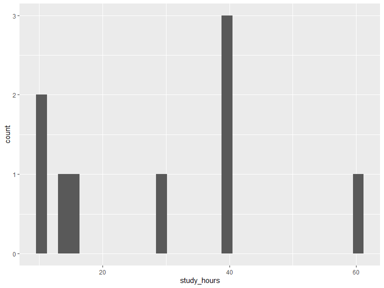

# Min, max, median & mean hours/day out
kable(t(as.matrix(summary(veritas_main$study_hours[veritas_main$studying == 1]))),
  caption = "study hours/week",
  digits = 1
) %>%
  kable_styling(bootstrap_options = "striped", full_width = T, position = "left")

study hours/week

Min.	1st Qu.	Median	Mean	3rd Qu.	Max.
10	14	30	28.8	40	60

3.3 Section 3: Shopping activities

3.3.1 In Date of Previous Data Collection Wave, you reported shopping at these locations. Do you still visit these places?

shop_lut <- data.frame(
  location_category_code = c(5, 6, 7, 8, 9, 10),
  location_category = factor(c(
    " 5 [Supermarket]",
    " 6 [Public/farmer’s market]",
    " 7 [Bakery]",
    " 8 [Specialty food store]",
    " 9 [Convenience store/Dépanneur]",
    "10 [Liquor store/SAQ]"
  ))
)
shop_location <- locations[locations$location_category %in% shop_lut$location_category_code, ] %>%
  filter(location_current == 1) %>%
  dplyr::rename(location_category_code = location_category) %>%
  inner_join(shop_lut, by = "location_category_code")

# map
bm + geom_sf(data = shop_location, inherit.aes = FALSE, aes(color = location_category), size = 1.5, alpha = .3) +
  scale_color_brewer(palette = "Accent") +
  theme(legend.position = "bottom", legend.text = element_text(size = 8), legend.title = element_blank())

# compute number of shopping locations by category
ggplot(data = shop_location) +
  geom_histogram(aes(x = location_category), stat = "count") +
  scale_x_discrete(labels = function(lbl) str_wrap(lbl, width = 20)) +
  labs(x = "Shopping locations by categories")

.location_category_cnt <- as.data.frame(shop_location[c("location_category")]) %>%
  group_by(location_category) %>%
  dplyr::count() %>%
  arrange(location_category)
kable(.location_category_cnt, caption = "Shopping locations by categories") %>% kable_styling(bootstrap_options = "striped", full_width = T, position = "left")

Shopping locations by categories

location_category	n
5 [Supermarket]	155
6 [Public/farmer’s market]	5
7 [Bakery]	14
8 [Specialty food store]	29
9 [Convenience store/Dépanneur]	18
10 [Liquor store/SAQ]	25

# compute statistics on shopping locations by participants and categories
# > one needs to account for participants who did not report location for some categories
.loc_iid_category_cnt <- as.data.frame(shop_location[c("interact_id", "location_category")]) %>%
  group_by(interact_id, location_category) %>%
  dplyr::count()

# (cont'd) simulate SQL JOIN TABLE ON TRUE to build list of all combination iid/shopping categ
.dummy <- data_frame(
  interact_id = character(),
  location_category = character()
)
for (iid in as.vector(veritas_main$interact_id)) {
  .dmy <- data_frame(
    interact_id = as.character(iid),
    location_category = shop_lut$location_category
  )
  .dummy <- rbind(.dummy, .dmy)
}

# (cont'd) find iid/categ combination without match in veritas locations
.no_shop_iid <- dplyr::setdiff(.dummy, .loc_iid_category_cnt[c("location_category", "interact_id")]) %>%
  mutate(n = 0)
.loc_iid_category_cnt <- bind_rows(.loc_iid_category_cnt, .no_shop_iid)

.location_category_cnt <- .loc_iid_category_cnt %>%
  group_by(location_category) %>%
  dplyr::summarise(min = min(n), mean = round(mean(n), 2), median = median(n), max = max(n)) %>%
  arrange(location_category)
kable(.location_category_cnt, caption = "Number of shopping locations by participant and category") %>% kable_styling(bootstrap_options = "striped", full_width = T, position = "left")

Number of shopping locations by participant and category

location_category	min	mean	median	max
5 [Supermarket]	0	2.46	2	5
6 [Public/farmer’s market]	0	0.08	0	1
7 [Bakery]	0	0.22	0	4
8 [Specialty food store]	0	0.46	0	3
9 [Convenience store/Dépanneur]	0	0.29	0	4
10 [Liquor store/SAQ]	0	0.40	0	3

3.3.2 Thinking about the places where you shop, are there other supermarkets, farmers markets, bakeries, specialty stores, convenience stores or liquor stores you visit at least once per month?

# extract and recode
.grp_shopping <- veritas_main[c("interact_id", "grp_shopping_new")] %>% dplyr::rename(grp_shopping_new_code = grp_shopping_new)
.grp_shopping$grp_shopping_new <- factor(ifelse(.grp_shopping$grp_shopping_new_code == 1, "1 [Yes]",
  ifelse(.grp_shopping$grp_shopping_new_code == 2, "2 [No]", "N/A")
))

# histogram of answers
ggplot(data = .grp_shopping) +
  geom_histogram(aes(x = grp_shopping_new), stat = "count") +
  scale_x_discrete(labels = function(lbl) str_wrap(lbl, width = 20)) +
  labs(x = "grp_shopping_new")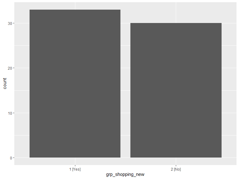

.grp_shopping_cnt <- .grp_shopping %>%
  group_by(grp_shopping_new) %>%
  dplyr::count() %>%
  arrange(grp_shopping_new)
kable(.grp_shopping_cnt, caption = "New shopping places") %>% kable_styling(bootstrap_options = "striped", full_width = T, position = "left")

New shopping places

grp_shopping_new	n
1 [Yes]	33
2 [No]	30

3.4 Section 4: Services

3.4.1 In Date of Previous Data Collection Wave, you reported using services at these locations. Do you still visit these places?

serv_lut <- data.frame(
  location_category_code = c(11, 12, 13, 14, 15),
  location_category = factor(c(
    "11 [Bank]",
    "12 [Hair salon/barbershop]",
    "13 [Post office]",
    "14 [Drugstore]",
    "15 Doctor/healthcare provider]"
  ))
)
serv_location <- locations[locations$location_category %in% serv_lut$location_category_code, ] %>%
  filter(location_current == 1) %>%
  dplyr::rename(location_category_code = location_category) %>%
  inner_join(serv_lut, by = "location_category_code")

# map
bm + geom_sf(data = serv_location, inherit.aes = FALSE, aes(color = location_category), size = 1.5, alpha = .3) +
  scale_color_brewer(palette = "Accent") +
  theme(legend.position = "bottom", legend.text = element_text(size = 8), legend.title = element_blank())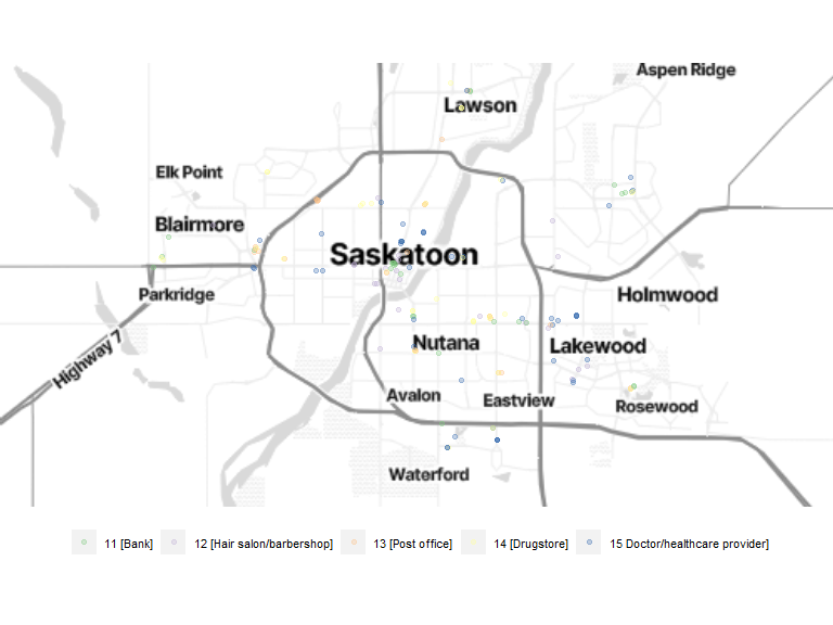

# compute number of shopping locations by category
ggplot(data = serv_location) +
  geom_histogram(aes(x = location_category), stat = "count") +
  scale_x_discrete(labels = function(lbl) str_wrap(lbl, width = 20)) +
  labs(x = "Service locations by categories")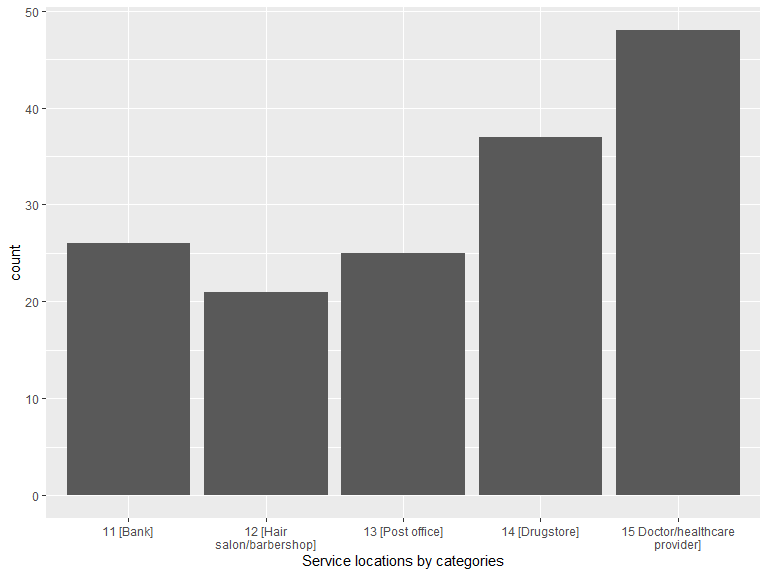

.location_category_cnt <- as.data.frame(serv_location[c("location_category")]) %>%
  group_by(location_category) %>%
  dplyr::count() %>%
  arrange(location_category)
kable(.location_category_cnt, caption = "Shopping locations by categories") %>% kable_styling(bootstrap_options = "striped", full_width = T, position = "left")

Shopping locations by categories

location_category	n
11 [Bank]	26
12 [Hair salon/barbershop]	21
13 [Post office]	25
14 [Drugstore]	37
15 Doctor/healthcare provider]	48

# compute statistics on shopping locations by participants and categories
# > one needs to account for participants who did not report location for some categories
.loc_iid_category_cnt <- as.data.frame(serv_location[c("interact_id", "location_category")]) %>%
  group_by(interact_id, location_category) %>%
  dplyr::count()

# (cont'd) simulate SQL JOIN TABLE ON TRUE
.dummy <- data_frame(
  interact_id = character(),
  location_category = character()
)
for (iid in as.vector(veritas_main$interact_id)) {
  .dmy <- data_frame(
    interact_id = as.character(iid),
    location_category = serv_lut$location_category
  )
  .dummy <- rbind(.dummy, .dmy)
}

# (cont'd) find iid/categ combination without match in veritas locations
.no_serv_iid <- dplyr::setdiff(.dummy, .loc_iid_category_cnt[c("location_category", "interact_id")]) %>%
  mutate(n = 0)
.loc_iid_category_cnt <- bind_rows(.loc_iid_category_cnt, .no_serv_iid)

.location_category_cnt <- .loc_iid_category_cnt %>%
  group_by(location_category) %>%
  dplyr::summarise(min = min(n), mean = round(mean(n), 2), median = median(n), max = max(n)) %>%
  arrange(location_category)
kable(.location_category_cnt, caption = "Number of shopping locations by participant and category") %>% kable_styling(bootstrap_options = "striped", full_width = T, position = "left")

Number of shopping locations by participant and category

location_category	min	mean	median	max
11 [Bank]	0	0.41	0	1
12 [Hair salon/barbershop]	0	0.33	0	1
13 [Post office]	0	0.40	0	1
14 [Drugstore]	0	0.59	1	1
15 Doctor/healthcare provider]	0	0.76	1	4

3.4.2 Thinking about the places where you use services, are there other banks, hair salons, post offices, drugstores, doctors or other healthcare providers you visit at least once per month?

NB: Variable grp_services_new has not been properly recorded in Saskatoon wave 2 for returning participants.

# extract and recode
.grp_services <- veritas_main[c("interact_id", "grp_services_new")] %>% dplyr::rename(grp_services_new_code = grp_services_new)
.grp_services$grp_services_new <- factor(ifelse(.grp_services$grp_services_new_code == 1, "1 [Yes]",
  ifelse(.grp_services$grp_services_new_code == 2, "2 [No]", "N/A")
))

# histogram of answers
ggplot(data = .grp_services) +
  geom_histogram(aes(x = grp_services_new), stat = "count") +
  scale_x_discrete(labels = function(lbl) str_wrap(lbl, width = 20)) +
  labs(x = "grp_services_new")

.grp_services_cnt <- .grp_services %>%
  group_by(grp_services_new) %>%
  dplyr::count() %>%
  arrange(grp_services_new)
kable(.grp_services_cnt, caption = "New services places") %>% kable_styling(bootstrap_options = "striped", full_width = T, position = "left")

3.5 Section 5: Transportation

3.5.1 In Date of Previous Data Collection Wave, you reported accessing these public transit stops from your home. Do you still access these places?

transp_location <- locations[locations$location_category == 16, ] %>% filter(location_current == 1)

bm + geom_sf(data = transp_location, inherit.aes = FALSE, color = "blue", size = 1.8, alpha = .3)

3.5.2 Are there other public transit stops you access from your home at least once per month?

NB: Variable grp_ptransit_new has not been properly recorded in Saskatoon wave 2 for returning participants.

# extract and recode
.grp_ptransit <- veritas_main[c("interact_id", "grp_ptransit_new")] %>% dplyr::rename(grp_ptransit_new_code = grp_ptransit_new)
.grp_ptransit$grp_ptransit_new <- factor(ifelse(.grp_ptransit$grp_ptransit_new_code == 1, "1 [Yes]",
  ifelse(.grp_ptransit$grp_ptransit_new_code == 2, "2 [No]", "N/A")
))

# histogram of answers
ggplot(data = .grp_ptransit) +
  geom_histogram(aes(x = grp_ptransit_new), stat = "count") +
  scale_x_discrete(labels = function(lbl) str_wrap(lbl, width = 20)) +
  labs(x = "grp_ptransit_new")

.grp_ptransit_cnt <- .grp_ptransit %>%
  group_by(grp_ptransit_new) %>%
  dplyr::count() %>%
  arrange(grp_ptransit_new)
kable(.grp_ptransit_cnt, caption = "New transit places") %>% kable_styling(bootstrap_options = "striped", full_width = T, position = "left")

3.6 Section 6: Leisure activities

3.6.1 In Date of Previous Data Collection Wave, you reported doing leisure activities at these locations. Do you still visit these places?

leisure_lut <- data.frame(
  location_category_code = c(17, 18, 19, 20, 21, 22, 23, 24),
  location_category = factor(c(
    "17 [Leisure-time physical activity]",
    "18 [Park]",
    "19 [Cultural activity]",
    "20 [Volunteering place]",
    "21 [Religious or spiritual activity]",
    "22 [Restaurant, café, bar, etc. ]",
    "23 [Take-out]",
    "24 [Walk]"
  ))
)
leisure_location <- locations[locations$location_category %in% leisure_lut$location_category_code, ] %>%
  dplyr::rename(location_category_code = location_category) %>%
  inner_join(leisure_lut, by = "location_category_code")

# map
bm + geom_sf(data = leisure_location, inherit.aes = FALSE, aes(color = location_category), size = 1.5, alpha = .3) +
  scale_color_brewer(palette = "Accent") +
  theme(legend.position = "bottom", legend.text = element_text(size = 8), legend.title = element_blank())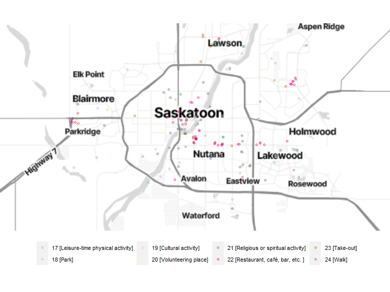

# compute number of shopping locations by category
ggplot(data = leisure_location) +
  geom_histogram(aes(x = location_category), stat = "count") +
  scale_x_discrete(labels = function(lbl) str_wrap(lbl, width = 20)) +
  labs(x = "Leisure locations by categories")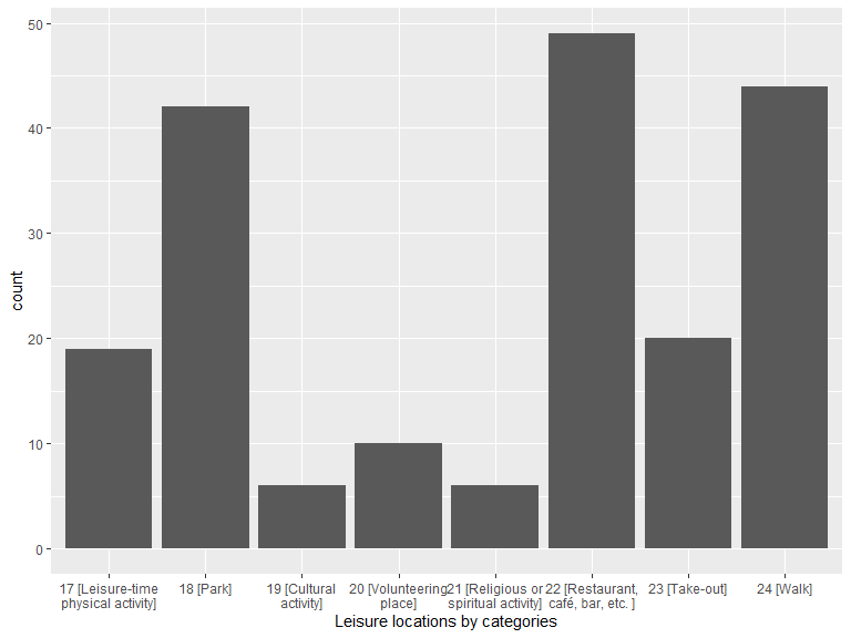

.location_category_cnt <- as.data.frame(leisure_location[c("location_category")]) %>%
  group_by(location_category) %>%
  dplyr::count() %>%
  arrange(location_category)
kable(.location_category_cnt, caption = "Shopping locations by categories") %>% kable_styling(bootstrap_options = "striped", full_width = T, position = "left")

Shopping locations by categories

location_category	n
17 [Leisure-time physical activity]	19
18 [Park]	42
19 [Cultural activity]	6
20 [Volunteering place]	10
21 [Religious or spiritual activity]	6
22 [Restaurant, café, bar, etc. ]	49
23 [Take-out]	20
24 [Walk]	44

# compute statistics on shopping locations by participants and categories
# > one needs to account for participants who did not report location for some categories
.loc_iid_category_cnt <- as.data.frame(leisure_location[c("interact_id", "location_category")]) %>%
  group_by(interact_id, location_category) %>%
  dplyr::count()

# (cont'd) simulate SQL JOIN TABLE ON TRUE
.dummy <- data_frame(
  interact_id = character(),
  location_category = character()
)
for (iid in as.vector(veritas_main$interact_id)) {
  .dmy <- data_frame(
    interact_id = as.character(iid),
    location_category = leisure_lut$location_category
  )
  .dummy <- rbind(.dummy, .dmy)
}

# (cont'd) find iid/categ combination without match in veritas locations
.no_leisure_iid <- dplyr::setdiff(.dummy, .loc_iid_category_cnt[c("location_category", "interact_id")]) %>%
  mutate(n = 0)

.loc_iid_category_cnt <- bind_rows(.loc_iid_category_cnt, .no_leisure_iid)

.location_category_cnt <- .loc_iid_category_cnt %>%
  group_by(location_category) %>%
  dplyr::summarise(min = min(n), mean = round(mean(n), 2), median = median(n), max = max(n)) %>%
  arrange(location_category)
kable(.location_category_cnt, caption = "Number of leisure locations by participant and category") %>% kable_styling(bootstrap_options = "striped", full_width = T, position = "left")

Number of leisure locations by participant and category

location_category	min	mean	median	max
17 [Leisure-time physical activity]	0	0.30	0	4
18 [Park]	0	0.67	0	3
19 [Cultural activity]	0	0.10	0	2
20 [Volunteering place]	0	0.16	0	2
21 [Religious or spiritual activity]	0	0.10	0	2
22 [Restaurant, café, bar, etc. ]	0	0.78	0	4
23 [Take-out]	0	0.32	0	2
24 [Walk]	0	0.70	0	4

3.6.2 Thinking about the places where you do leisure activities, are there other parks, gyms, movie theaters, concert halls, churchs, temples, restaurants, cafés, bars or any places where you do leisure activities and that you visit at least once per month?

NB: Variable grp_leisure_new has not been properly recorded in Saskatoon wave 2 for returning participants.

# extract and recode
.grp_leisure <- veritas_main[c("interact_id", "grp_leisure_new")] %>% dplyr::rename(grp_leisure_new_code = grp_leisure_new)
.grp_leisure$grp_leisure_new <- factor(ifelse(.grp_leisure$grp_leisure_new_code == 1, "1 [Yes]",
  ifelse(.grp_leisure$grp_leisure_new_code == 2, "2 [No]", "N/A")
))

# histogram of answers
ggplot(data = .grp_leisure) +
  geom_histogram(aes(x = grp_leisure_new), stat = "count") +
  scale_x_discrete(labels = function(lbl) str_wrap(lbl, width = 20)) +
  labs(x = "grp_leisure_new")

.grp_leisure_cnt <- .grp_leisure %>%
  group_by(grp_leisure_new) %>%
  dplyr::count() %>%
  arrange(grp_leisure_new)
kable(.grp_leisure_cnt, caption = "New leisure places") %>% kable_styling(bootstrap_options = "striped", full_width = T, position = "left")

3.7 Section 7: Other places/activities

3.7.1 Here are the other places you reported regularly visiting in Date of Previous Data Collection Wave. Do you still visit these places?

other_location <- locations[locations$location_category == 25, ] %>% filter(location_current == 1)

bm + geom_sf(data = other_location, inherit.aes = FALSE, color = "blue", size = 1.8, alpha = .3)

3.7.2 Are there other places that you go to at least once per month that we have not mentioned? For example: a mall, a daycare, a hardware store, or a community center.

NB: Variable other_new has not been properly recorded in Saskatoon wave 2 for returning participants.

# extract and recode
.other <- veritas_main[c("interact_id", "other_new")] %>% dplyr::rename(other_new_code = other_new)
.other$other_new <- factor(ifelse(.other$other_new_code == 1, "1 [Yes]",
  ifelse(.other$other_new_code == 2, "2 [No]", "N/A")
))

# histogram of answers
ggplot(data = .other) +
  geom_histogram(aes(x = other_new), stat = "count") +
  scale_x_discrete(labels = function(lbl) str_wrap(lbl, width = 20)) +
  labs(x = "other_new")

.other_cnt <- .other %>%
  group_by(other_new) %>%
  dplyr::count() %>%
  arrange(other_new)
kable(.other_cnt, caption = "New other places") %>% kable_styling(bootstrap_options = "striped", full_width = T, position = "left")

3.8 Section 8: Areas of change

3.8.1 Can you locate areas where you have noticed an improvement of the urban environment?

# extract and recode
.improv <- veritas_main[c("interact_id", "improvement_none")] %>% dplyr::rename(improvement_none_code = improvement_none)
.improv$improvement_none <- factor(ifelse(.improv$improvement_none_code == 1, "1 [TRUE]",
  ifelse(.improv$improvement_none_code == 0, "0 [FALSE]", "N/A")
))

# histogram of answers
ggplot(data = .improv) +
  geom_histogram(aes(x = improvement_none), stat = "count") +
  scale_x_discrete(labels = function(lbl) str_wrap(lbl, width = 20)) +
  labs(x = "improvement_none")

.improv_cnt <- .improv %>%
  group_by(improvement_none) %>%
  dplyr::count() %>%
  arrange(improvement_none)
kable(.improv_cnt, caption = "No area of improvement") %>% kable_styling(bootstrap_options = "striped", full_width = T, position = "left")

No area of improvement

improvement_none	n
0 [FALSE]	19
1 [TRUE]	44

# polgon extraction
improv <- poly_geom[poly_geom$area_type == "improvement", ]

# Map
bm + geom_sf(data = improv, inherit.aes = FALSE, fill = alpha("blue", 0.3), color = alpha("blue", 0.5))

# Min, max, median & mean area of PRN
improv <- improv %>%
  mutate(area_m2 = st_area(.))
kable(t(as.matrix(summary(improv$area_m2))),
  caption = "Area (in square meters) of the perceived improvement areas",
  digits = 1
) %>% kable_styling(bootstrap_options = "striped", full_width = T, position = "left")

Area (in square meters) of the perceived improvement areas

Min.	1st Qu.	Median	Mean	3rd Qu.	Max.
6263.4	25218.5	93234.7	306373.6	175202.1	2126591

3.8.2 Can you locate areas where you have noticed a deterioration of the urban environment?

# extract and recode
.deter <- veritas_main[c("interact_id", "deterioration_none")] %>% dplyr::rename(deterioration_none_code = deterioration_none)
.deter$deterioration_none <- factor(ifelse(.deter$deterioration_none_code == 1, "1 [TRUE]",
  ifelse(.deter$deterioration_none_code == 0, "0 [FALSE]", "N/A")
))

# histogram of answers
ggplot(data = .deter) +
  geom_histogram(aes(x = deterioration_none), stat = "count") +
  scale_x_discrete(labels = function(lbl) str_wrap(lbl, width = 20)) +
  labs(x = "deterioration_none")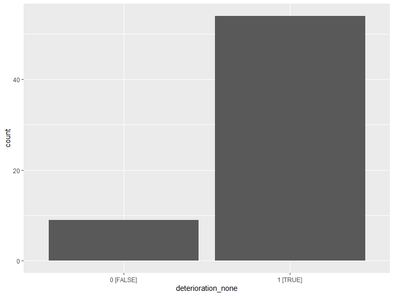

.deter_cnt <- .deter %>%
  group_by(deterioration_none) %>%
  dplyr::count() %>%
  arrange(deterioration_none)
kable(.deter_cnt, caption = "No area of deterioration") %>% kable_styling(bootstrap_options = "striped", full_width = T, position = "left")

No area of deterioration

deterioration_none	n
0 [FALSE]	9
1 [TRUE]	54

# polgon extraction
deter <- poly_geom[poly_geom$area_type == "deterioration", ]

# Map
bm + geom_sf(data = deter, inherit.aes = FALSE, fill = alpha("blue", 0.3), color = alpha("blue", 0.5))

# Min, max, median & mean area of PRN
deter <- deter %>%
  mutate(area_m2 = st_area(.))
kable(t(as.matrix(summary(deter$area_m2))),
  caption = "Area (in square meters) of the perceived deterioration areas",
  digits = 1
) %>%
  kable_styling(bootstrap_options = "striped", full_width = T, position = "left")

Area (in square meters) of the perceived deterioration areas

Min.	1st Qu.	Median	Mean	3rd Qu.	Max.
1625	12642.9	72128	199827.2	265169.7	951943.7

3.9 Section 9: Social contact

3.9.1 In Date of Previous Data Collection Wave, you reported visiting people at their home. Do you still visit these places?

visiting_location <- locations[locations$location_category == 26, ] %>% filter(location_current == 1)

bm + geom_sf(data = visiting_location, inherit.aes = FALSE, color = "blue", size = 1.8, alpha = .3)

3.9.2 Do you visit anyone else at his or her home at least once per month?

NB: Variable visiting_new has not been properly recorded in Saskatoon wave 2 for returning participants.

# extract and recode
.visiting <- veritas_main[c("interact_id", "visiting_new")] %>% dplyr::rename(visiting_code = visiting_new)
.visiting$visiting_new <- factor(ifelse(.visiting$visiting_code == 1, "1 [Yes]",
  ifelse(.visiting$visiting_code == 2, "2 [No]", "N/A")
))

# histogram of answers
ggplot(data = .visiting) +
  geom_histogram(aes(x = visiting_new), stat = "count") +
  scale_x_discrete(labels = function(lbl) str_wrap(lbl, width = 20)) +
  labs(x = "visiting_new")

.visiting_cnt <- .visiting %>%
  group_by(visiting_new) %>%
  dplyr::count() %>%
  arrange(visiting_new)
kable(.visiting_cnt, caption = "Social contact") %>% kable_styling(bootstrap_options = "striped", full_width = T, position = "left")

3.9.3 Great, we are almost done completing this questionnaire. You have documented all your activity places on a map, and specified with whom you generally do these activities. These last few questions concern the people you documented earlier.

# compute statistics on groups / participant
# > one needs to account for participants who did not report any group
.gr_iid_cnt <- as.data.frame(group[c("interact_id")]) %>%
  group_by(interact_id) %>%
  dplyr::count()

# (cont'd) find iid combination without match in veritas group
.no_gr_iid <- anti_join(veritas_main[c("interact_id")], .gr_iid_cnt, by = "interact_id") %>%
  mutate(n = 0)
.gr_iid_cnt <- bind_rows(.gr_iid_cnt, .no_gr_iid)

kable(t(as.matrix(summary(.gr_iid_cnt$n))),
  caption = "Number of groups per participant",
  digits = 1
) %>%
  kable_styling(bootstrap_options = "striped", full_width = T, position = "left")

Number of groups per participant

Min.	1st Qu.	Median	Mean	3rd Qu.	Max.
0	0	1	1.3	2	6

# compute statistics on people / participant
# > one needs to account for participants who did not report any group
.pl_iid_cnt <- as.data.frame(people[c("interact_id")]) %>%
  group_by(interact_id) %>%
  dplyr::count()

# (cont'd) find iid combination without match in veritas group
.no_pl_iid <- anti_join(veritas_main[c("interact_id")], .pl_iid_cnt, by = "interact_id") %>%
  mutate(n = 0)
.pl_iid_cnt <- bind_rows(.pl_iid_cnt, .no_pl_iid)

kable(t(as.matrix(summary(.pl_iid_cnt$n))),
  caption = "Number of people per participant",
  digits = 1
) %>%
  kable_styling(bootstrap_options = "striped", full_width = T, position = "left")

Number of people per participant

Min.	1st Qu.	Median	Mean	3rd Qu.	Max.
0	3	5	6.2	8	38

# histogram
.sc_iid_cnt <- .pl_iid_cnt %>% mutate(soc_type = "people")
.sc_iid_cnt <- .gr_iid_cnt %>%
  mutate(soc_type = "group") %>%
  bind_rows(.sc_iid_cnt)

ggplot(data = .sc_iid_cnt) +
  geom_histogram(aes(x = n, y = stat(count), fill = soc_type), position = "dodge") +
  labs(x = "Social network size by element type", fill = element_blank())

3.9.3.1 Among these people, who do you discuss important matters with?

# extract number of important people / participant
.n_important <- important %>% dplyr::count(interact_id)
.n_people <- people %>% dplyr::count(interact_id)

.n_people_imp <- left_join(veritas_main[c("interact_id")], .n_people, by = "interact_id") %>%
  left_join(.n_important, by = "interact_id") %>%
  mutate_all(~ replace(., is.na(.), 0)) %>%
  dplyr::rename(n_people = n.x, n_important = n.y) %>%
  mutate(pct = 100 * n_important / n_people)

kable(t(as.matrix(summary(.n_people_imp$n_important))),
  caption = "Number of important people per participant",
  digits = 1
) %>%
  kable_styling(bootstrap_options = "striped", full_width = T, position = "left")

Number of important people per participant

Min.	1st Qu.	Median	Mean	3rd Qu.	Max.
0	1	2	2.9	4	19

kable(t(as.matrix(summary(.n_people_imp$pct))),
  caption = "% of important people among social contact per participant",
  digits = 1
) %>%
  kable_styling(bootstrap_options = "striped", full_width = T, position = "left")

% of important people among social contact per participant

Min.	1st Qu.	Median	Mean	3rd Qu.	Max.	NA’s
11.1	33.3	50	55.8	80	100	3

3.9.3.2 Among these people, who do you like to socialize with?

# extract number of important people / participant
.n_socialize <- socialize %>% dplyr::count(interact_id)
.n_people <- people %>% dplyr::count(interact_id)

.n_people_soc <- left_join(veritas_main[c("interact_id")], .n_people, by = "interact_id") %>%
  left_join(.n_socialize, by = "interact_id") %>%
  mutate_all(~ replace(., is.na(.), 0)) %>%
  dplyr::rename(n_people = n.x, n_socialize = n.y) %>%
  mutate(pct = 100 * n_socialize / n_people)

kable(t(as.matrix(summary(.n_people_soc$n_socialize))),
  caption = "Number of people with whom to socialize per participant",
  digits = 1
) %>%
  kable_styling(bootstrap_options = "striped", full_width = T, position = "left")

Number of people with whom to socialize per participant

Min.	1st Qu.	Median	Mean	3rd Qu.	Max.
0	2	3	4.2	5	20

kable(t(as.matrix(summary(.n_people_soc$pct))),
  caption = "% of people with whom to  socialize among social contact per participant",
  digits = 1
) %>%
  kable_styling(bootstrap_options = "striped", full_width = T, position = "left")

% of people with whom to socialize among social contact per participant

Min.	1st Qu.	Median	Mean	3rd Qu.	Max.	NA’s
0	52	73.9	71.1	100	100	3

3.9.3.3 Among these people, who do you meet often with but do not necessarily feel close to?

# extract number of important people / participant
.n_not_close <- not_close %>% dplyr::count(interact_id)
.n_people <- people %>% dplyr::count(interact_id)

.n_people_not_close <- left_join(veritas_main[c("interact_id")], .n_people, by = "interact_id") %>%
  left_join(.n_not_close, by = "interact_id") %>%
  mutate_all(~ replace(., is.na(.), 0)) %>%
  dplyr::rename(n_people = n.x, n_not_close = n.y) %>%
  mutate(pct = 100 * n_not_close / n_people)

kable(t(as.matrix(summary(.n_people_not_close$n_not_close))),
  caption = "Number of not so close people per participant",
  digits = 1
) %>%
  kable_styling(bootstrap_options = "striped", full_width = T, position = "left")

Number of not so close people per participant

Min.	1st Qu.	Median	Mean	3rd Qu.	Max.
0	0	0	0.7	1	5

kable(t(as.matrix(summary(.n_people_not_close$pct))),
  caption = "% of not so close people among social contact per participant",
  digits = 1
) %>%
  kable_styling(bootstrap_options = "striped", full_width = T, position = "left")

% of not so close people among social contact per participant

Min.	1st Qu.	Median	Mean	3rd Qu.	Max.	NA’s
0	0	0	11.9	25	50	3

3.9.3.4 Among these people, who knows whom?

# extract number of who knows who relationships
.n_relat <- relationship %>%
  filter(relationship_type == 1) %>%
  dplyr::count(interact_id)
.n_people <- people %>% dplyr::count(interact_id)

.n_people_relat <- left_join(veritas_main[c("interact_id")], .n_people, by = "interact_id") %>%
  left_join(.n_relat, by = "interact_id") %>%
  mutate_all(~ replace(., is.na(.), 0)) %>%
  dplyr::rename(n_people = n.x, n_relat = n.y) %>%
  mutate(pct = 100 * n_relat * 2 / (n_people * (n_people - 1))) # potential number of relationships = N x (N -1) / 2

kable(t(as.matrix(summary(.n_people_relat$n_relat))),
  caption = "Number of relationships « who knows who » per participant",
  digits = 1
) %>%
  kable_styling(bootstrap_options = "striped", full_width = T, position = "left")

Number of relationships « who knows who » per participant

Min.	1st Qu.	Median	Mean	3rd Qu.	Max.
0	1	6	13.4	14.5	144

kable(t(as.matrix(summary(.n_people_relat$pct))),
  caption = "% of relationships « who knows who » per participant",
  digits = 1
) %>%
  kable_styling(bootstrap_options = "striped", full_width = T, position = "left")

% of relationships « who knows who » per participant

Min.	1st Qu.	Median	Mean	3rd Qu.	Max.	NA’s
0	39.6	66.7	63.8	100	100	7

3.10 Derived metrics

3.10.1 Existence of improvement and deterioration areas by participant

Combination of improvement and/or deterioration areas per participant

# cross tab of improvement vs deteriation areas
.improv <- improv[c("interact_id")] %>%
  mutate(improv = "Improvement")
.deter <- deter[c("interact_id")] %>%
  mutate(deter = "Deterioration")
.ct_impr_deter <- veritas_main[c("interact_id")] %>%
  transmute(interact_id = as.character(interact_id)) %>%
  left_join(.improv, by = "interact_id") %>%
  left_join(.deter, by = "interact_id") %>%
  mutate_all(~ replace(., is.na(.), "N/A"))

kable(table(.ct_impr_deter$improv, .ct_impr_deter$deter), caption = "Improvement vs. deterioration") %>%
  kable_styling(bootstrap_options = "striped", full_width = T, position = "left", row_label_position = "r") %>%
  column_spec(1, bold = T)

Improvement vs. deterioration

	Deterioration	N/A
Improvement	7	11
N/A	2	43

3.10.2 Transportation mode preferences

Based on the answers to the question Usually, how do you go there? (Check all that apply.).

# code  en
# 1 By car and you drive
# 2 By car and someone else drives
# 3 By taxi/Uber
# 4 On foot
# 5 By bike
# 6 By bus
# 7 By subway
# 8 By train
# 99    Other

loc_labels <- data.frame(location_category = c(2:26), description = c(
  " 2 [Other residence]",
  " 3 [Work]",
  " 4 [School/College/University]",
  " 5 [Supermarket]",
  " 6 [Public/farmer’s market]",
  " 7 [Bakery]",
  " 8 [Specialty food store]",
  " 9 [Convenience store/Dépanneur]",
  "10 [Liquor store/SAQ]",
  "11 [Bank]",
  "12 [Hair salon/barbershop]",
  "13 [Post office]",
  "14 [Drugstore]",
  "15 [Doctor/healthcare provider]",
  "16 [Public transit stop]",
  "17 [Leisure-time physical activity]",
  "18 [Park]",
  "19 [Cultural activity]",
  "20 [Volunteering place]",
  "21 [Religious/spiritual activity]",
  "22 [Restaurant, café, bar, etc.]",
  "23 [Take-out]",
  "24 [Walk]",
  "25 [Other place]",
  "26 [Social contact residence]"
))

# extract and summary stats
.tm <- locations %>%
  st_set_geometry(NULL) %>%
  filter(location_category != 1 & location_current == 1) %>%
  left_join(loc_labels)

.tm_grouped <- .tm %>%
  group_by(description) %>%
  dplyr::summarise(
    N = n(), "By car (driver)" = sum(location_tmode_1),
    "By car (passenger)" = sum(location_tmode_2),
    "By taxi/Uber" = sum(location_tmode_3),
    "On foot" = sum(location_tmode_4),
    "By bike" = sum(location_tmode_5),
    "By bus" = sum(location_tmode_6),
    "By train" = sum(location_tmode_7),
    "Other" = sum(location_tmode_99)
  )

kable(.tm_grouped, caption = "Transportation mode preferences") %>% kable_styling(bootstrap_options = "striped", full_width = T, position = "left")

Transportation mode preferences

description	N	By car (driver)	By car (passenger)	By taxi/Uber	On foot	By bike	By bus	By train	Other
2 [Other residence]	6	2	3	0	1	0	4	0	0
3 [Work]	67	18	10	2	9	5	17	0	27
4 [School/College/University]	12	3	2	0	3	1	3	0	4
5 [Supermarket]	155	88	41	3	30	7	21	0	3
6 [Public/farmer’s market]	5	3	0	0	1	2	0	0	0
7 [Bakery]	14	3	6	0	5	1	0	0	0
8 [Specialty food store]	29	17	5	0	7	2	0	0	1
9 [Convenience store/Dépanneur]	18	4	0	0	9	1	6	0	0
10 [Liquor store/SAQ]	25	15	2	0	5	3	4	0	0
11 [Bank]	26	14	4	0	7	2	2	0	2
12 [Hair salon/barbershop]	21	10	1	1	8	1	4	0	1
13 [Post office]	25	11	4	0	12	2	6	0	0
14 [Drugstore]	37	19	5	0	15	3	3	0	2
15 [Doctor/healthcare provider]	48	28	7	4	6	1	11	0	2
16 [Public transit stop]	52	0	0	0	46	0	10	0	1
17 [Leisure-time physical activity]	19	10	2	0	8	3	0	0	0
18 [Park]	42	4	2	0	35	5	0	0	0
19 [Cultural activity]	6	3	0	0	2	0	1	0	0
20 [Volunteering place]	10	4	1	0	2	1	1	0	3
21 [Religious/spiritual activity]	6	2	2	0	1	0	1	0	2
22 [Restaurant, café, bar, etc.]	49	17	13	1	17	3	7	0	2
23 [Take-out]	20	10	6	0	3	0	2	0	2
24 [Walk]	44	3	4	0	41	4	1	0	0
25 [Other place]	44	19	13	0	14	7	7	0	0

# graph
.tm1 <- .tm %>%
  filter(location_tmode_1 == 1) %>%
  mutate(tm = "[1] By car (driver)")
.tm2 <- .tm %>%
  filter(location_tmode_2 == 1) %>%
  mutate(tm = "[2] By car (passenger)")
.tm3 <- .tm %>%
  filter(location_tmode_3 == 1) %>%
  mutate(tm = "[3] By taxi/Uber")
.tm4 <- .tm %>%
  filter(location_tmode_4 == 1) %>%
  mutate(tm = "[4] On foot")
.tm5 <- .tm %>%
  filter(location_tmode_5 == 1) %>%
  mutate(tm = "[5] By bike")
.tm6 <- .tm %>%
  filter(location_tmode_6 == 1) %>%
  mutate(tm = "[6] By bus")
# .tm7 <- .tm %>%                       # Empty dataframe -> error when creating tm col.
#   filter(location_tmode_7 == 1) %>%
#   mutate(tm = "[7] By train")
.tm99 <- .tm %>%
  filter(location_tmode_99 == 1) %>%
  mutate(tm = "[99] Other")
.tm <- bind_rows(.tm1, .tm2) %>%
  bind_rows(.tm3) %>%
  bind_rows(.tm4) %>%
  bind_rows(.tm5) %>%
  bind_rows(.tm6) %>%
  #  bind_rows(.tm7) %>%
  bind_rows(.tm99)

# histogram of answers
ggplot(data = .tm) +
  geom_bar(aes(x = fct_rev(description), fill = tm), position = "fill") +
  scale_fill_brewer(palette = "Set3", name = "Transport modes") +
  scale_y_continuous(labels = percent) +
  labs(y = "Proportion of transportation mode by location category", x = element_blank()) +
  coord_flip() +
  theme(legend.position = "bottom", legend.justification = c(0, 0), legend.text = element_text(size = 8)) +
  guides(fill = guide_legend(nrow = 3))

3.10.3 Visiting places alone

Based on the answers to the question Do you usually go to this place alone or with other people?.

loc_labels <- data.frame(location_category = c(2:26), description = c(
  " 2 [Other residence]",
  " 3 [Work]",
  " 4 [School/College/University]",
  " 5 [Supermarket]",
  " 6 [Public/farmer’s market]",
  " 7 [Bakery]",
  " 8 [Specialty food store]",
  " 9 [Convenience store/Dépanneur]",
  "10 [Liquor store/SAQ]",
  "11 [Bank]",
  "12 [Hair salon/barbershop]",
  "13 [Post office]",
  "14 [Drugstore]",
  "15 [Doctor/healthcare provider]",
  "16 [Public transit stop]",
  "17 [Leisure-time physical activity]",
  "18 [Park]",
  "19 [Cultural activity]",
  "20 [Volunteering place]",
  "21 [Religious/spiritual activity]",
  "22 [Restaurant, café, bar, etc.]",
  "23 [Take-out]",
  "24 [Walk]",
  "25 [Other place]",
  "26 [Social contact residence]"
))

# extract and summary stats
.alone <- locations %>%
  st_set_geometry(NULL) %>%
  filter(location_category != 1 & location_current == 1) %>%
  left_join(loc_labels) %>%
  mutate(location_alone_recode = case_when(
    location_alone2 == 1 ~ 1,
    location_alone2 == 2 ~ 0
  ))

.alone_grouped <- .alone %>%
  group_by(description) %>%
  dplyr::summarise(
    N = n(), "Visited alone" = sum(location_alone_recode),
    "Visited alone (%)" = round(sum(location_alone_recode) * 100.0 / n(), digits = 1)
  )

kable(.alone_grouped, caption = "Visiting places alone") %>% kable_styling(bootstrap_options = "striped", full_width = T, position = "left")

Visiting places alone

description	N	Visited alone	Visited alone (%)
2 [Other residence]	6	1	16.7
3 [Work]	67	32	47.8
4 [School/College/University]	12	6	50.0
5 [Supermarket]	155	100	64.5
6 [Public/farmer’s market]	5	4	80.0
7 [Bakery]	14	6	42.9
8 [Specialty food store]	29	20	69.0
9 [Convenience store/Dépanneur]	18	16	88.9
10 [Liquor store/SAQ]	25	18	72.0
11 [Bank]	26	26	100.0
12 [Hair salon/barbershop]	21	19	90.5
13 [Post office]	25	22	88.0
14 [Drugstore]	37	32	86.5
15 [Doctor/healthcare provider]	48	43	89.6
16 [Public transit stop]	52	49	94.2
17 [Leisure-time physical activity]	19	7	36.8
18 [Park]	42	15	35.7
19 [Cultural activity]	6	4	66.7
20 [Volunteering place]	10	4	40.0
21 [Religious/spiritual activity]	6	4	66.7
22 [Restaurant, café, bar, etc.]	49	17	34.7
23 [Take-out]	20	13	65.0
24 [Walk]	44	13	29.5
25 [Other place]	44	28	63.6

# histogram of answers
ggplot(data = .alone) +
  geom_bar(aes(x = fct_rev(description), fill = factor(location_alone2)), position = "fill") +
  scale_fill_brewer(palette = "Set3", name = "Visiting places", labels = c("N/A", "Alone", "With someone")) +
  scale_y_continuous(labels = percent) +
  labs(y = "Proportion of places visited alone", x = element_blank()) +
  coord_flip()

3.10.4 Visit frequency

Based on the answers to the question How often do you go there?.

loc_labels <- data.frame(location_category = c(2:26), description = c(
  " 2 [Other residence]",
  " 3 [Work]",
  " 4 [School/College/University]",
  " 5 [Supermarket]",
  " 6 [Public/farmer’s market]",
  " 7 [Bakery]",
  " 8 [Specialty food store]",
  " 9 [Convenience store/Dépanneur]",
  "10 [Liquor store/SAQ]",
  "11 [Bank]",
  "12 [Hair salon/barbershop]",
  "13 [Post office]",
  "14 [Drugstore]",
  "15 [Doctor/healthcare provider]",
  "16 [Public transit stop]",
  "17 [Leisure-time physical activity]",
  "18 [Park]",
  "19 [Cultural activity]",
  "20 [Volunteering place]",
  "21 [Religious/spiritual activity]",
  "22 [Restaurant, café, bar, etc.]",
  "23 [Take-out]",
  "24 [Walk]",
  "25 [Other place]",
  "26 [Social contact residence]"
))

# extract and summary stats
.freq <- locations %>%
  st_set_geometry(NULL) %>%
  filter(location_category != 1 & location_current == 1) %>%
  left_join(loc_labels)

.freq_grouped <- .freq %>%
  group_by(description) %>%
  dplyr::summarise(
    N = n(), min = min(location_freq_visit),
    max = max(location_freq_visit),
    mean = mean(location_freq_visit),
    median = median(location_freq_visit),
    sd = sd(location_freq_visit)
  )

kable(.freq_grouped, caption = "Visit frequency (expressed in times/year)") %>% kable_styling(bootstrap_options = "striped", full_width = T, position = "left")

Visit frequency (expressed in times/year)

description	N	min	max	mean	median	sd
2 [Other residence]	6	24	364	146.666667	130	136.976884
3 [Work]	67	0	365	196.328358	260	138.880959
4 [School/College/University]	12	0	1040	269.083333	312	294.441060
5 [Supermarket]	155	0	260	34.819355	24	38.644815
6 [Public/farmer’s market]	5	1	52	33.800000	52	25.223005
7 [Bakery]	14	6	104	26.142857	24	25.059490
8 [Specialty food store]	29	2	24	10.965517	12	7.193662
9 [Convenience store/Dépanneur]	18	2	260	65.388889	18	83.981188
10 [Liquor store/SAQ]	25	1	156	22.880000	12	34.604094
11 [Bank]	26	0	12	6.500000	4	4.925444
12 [Hair salon/barbershop]	21	1	12	5.619048	5	4.443829
13 [Post office]	25	2	52	11.040000	5	12.306773
14 [Drugstore]	37	1	104	19.378378	12	22.395872
15 [Doctor/healthcare provider]	48	0	48	5.791667	2	8.039684
16 [Public transit stop]	52	0	1040	125.096154	50	193.168448
17 [Leisure-time physical activity]	19	12	364	85.263158	36	101.998280
18 [Park]	42	2	260	84.428571	52	81.751898
19 [Cultural activity]	6	0	104	39.000000	12	50.592490
20 [Volunteering place]	10	12	156	69.600000	52	56.480478
21 [Religious/spiritual activity]	6	8	364	157.333333	78	162.946208
22 [Restaurant, café, bar, etc.]	49	0	208	22.000000	12	32.348364
23 [Take-out]	20	1	52	13.750000	12	11.728844
24 [Walk]	44	2	936	125.409091	52	156.651341
25 [Other place]	44	0	156	27.113636	12	29.405122

# graph
ggplot(data = .freq) +
  geom_boxplot(aes(x = fct_rev(description), y = location_freq_visit)) +
  scale_y_continuous(limits = c(0, 365)) +
  labs(y = "Visits/year (Frequency over 1 visit/day not shown)", x = element_blank()) +
  coord_flip()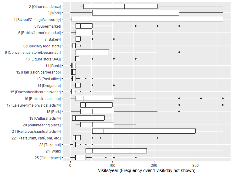

3.10.5 Spatial indicators: Camille Perchoux’s toolbox

Below is a list of indicators proposed by Camille Perchoux in her paper Assessing patterns of spatial behavior in health studies: Their socio-demographic determinants and associations with transportation modes (the RECORD Cohort Study).

-- Reading Camille tbx indics from Essence table
SELECT interact_id,
  n_acti_places, n_weekly_vst, n_acti_types,
  cvx_perimeter, cvx_surface,
  min_length, max_length, median_length, 
  pct_visits_neighb, 
  n_acti_prn, pct_visits_prn, prn_area_km2
FROM essence_table.essence_perchoux_tbx
WHERE city_id = 'Saskatoon' AND wave_id = 2 AND status = 'return'

3.10.5.1 Indicators related to the lifestyle

Indicators	Measurement approach
Number of activity places (n_acti_places)	Count of activity places
Number of visits to places per week (n_weekly_vst)	Number of activity places per individual multiplied by the frequency of visit per week to each location, excluding the residence
Number of activity types (n_acti_types)	6 types of activities considered: 1-Residential; 2-Occupation; 3-Shopping activities; 4-Services; 5-Transportation; 6-Leisure activities (NB original categories were as follow: 1-Residential; 2-work; 3-food and other services; 4-transport station/stop; 5-recreational activity; 6-social activity)

LLindic <- ess.tab.camille %>%
  select("interact_id", "n_acti_places", "n_weekly_vst", "n_acti_types")
.llmtx <- as.matrix(summary(LLindic[c("n_acti_places", "n_weekly_vst", "n_acti_types")], digits = 1))
.llmtx <- apply(.llmtx, 1:2, function(x) strsplit(as.character(x), ":")[[1]][2])
rownames(.llmtx) <- c("Min.   ", "1st Qu.", "Median ", "Mean   ", "3rd Qu.", "Max.   ")
kable(.llmtx, caption = "Lifestyle statistics") %>% kable_styling(bootstrap_options = "striped", full_width = T, position = "left")

Lifestyle statistics

	n_acti_places	n_weekly_vst	n_acti_types
Min.	2	0.5	2
1st Qu.	9	8.3	4
Median	13	11.8	5
Mean	13	14.8	5
3rd Qu.	17	17.6	6
Max.	26	65.6	6

3.10.5.2 Indicators related to the geometry of the activity space

Indicators	Measurement approach
Perimeter of the convex hull (cvx_perimeter)	Perimeter of the smallest polygon containing all the activity locations of the participant (unit: km)
Surface of the convex hull (cvx_surface)	Surface of the smallest polygon containing all the activity locations of the participant (unit: km2)
Minimal road network distance from the residence to an activity place (min_length)	Minimal distance from the residence to an activity place using the road network (in meters)
Maximal road network distance from the residence to an activity place (max_length)	Maximal distance from the residence to an activity place using the road network (in meters)
Median road network distance from the residence to all activity places (median_length)	Median distance from home to all activity places using the road network (in meters)

ASindic <- ess.tab.camille %>%
  select("interact_id", "cvx_perimeter", "cvx_surface", "min_length", "max_length", "median_length")
.asmtx <- as.matrix(summary(ASindic[c("cvx_perimeter", "cvx_surface", "min_length", "max_length", "median_length")], digits = 1))
.asmtx <- apply(.asmtx, 1:2, function(x) strsplit(as.character(x), ":")[[1]][2])
rownames(.asmtx) <- c("Min.   ", "1st Qu.", "Median ", "Mean   ", "3rd Qu.", "Max.   ")
.asmtx[is.na(.asmtx)] <- 0
kable(.asmtx, caption = "Activity space statistics") %>% kable_styling(bootstrap_options = "striped", full_width = T, position = "left")

Activity space statistics

	cvx_perimeter	cvx_surface	min_length	max_length	median_length
Min.	2	0	0	1e+03	101
1st Qu.	14	7	29	6e+03	1228
Median	19	15	126	8e+03	2040
Mean	36	42	334	1e+04	2124
3rd Qu.	24	27	317	1e+04	2894
Max.	480	784	2873	2e+05	5603

3.10.5.3 Indicators related to the importance of the residential neighborhood

Indicators	Measurement approach
Percentage of visits to places in the residential neighborhood (pct_visits_neighb)	Count of visits to places within the 500 m road network buffer centered on the residence divided by the total number of visits to places
Number of activity locations in the PRN (n_acti_prn)	Count of activity locations in the PRN
Percentage of visits in the PRN (pct_visits_prn)	Count of visits to places in the PRN divided by the total number of visits to places
Surface of the PRN (prn_area_km2)	Unit: km2

RNindic <- ess.tab.camille %>%
  select("interact_id", "pct_visits_neighb", "n_acti_prn", "pct_visits_prn", "prn_area_km2")
RNindic <- RNindic[RNindic$interact_id %in% prn$interact_id, ]
.rnmtx <- as.matrix(summary(RNindic[c("pct_visits_neighb", "n_acti_prn", "pct_visits_prn", "prn_area_km2")], digits = 1))
.rnmtx <- apply(.rnmtx, 1:2, function(x) strsplit(as.character(x), ":")[[1]][2])
rownames(.rnmtx) <- c("Min.   ", "1st Qu.", "Median ", "Mean   ", "3rd Qu.", "Max.   ", "N/A.")
.rnmtx[is.na(.rnmtx)] <- 0
kable(.rnmtx, caption = "Residential neighbourhood statistics") %>% kable_styling(bootstrap_options = "striped", full_width = T, position = "left")

Residential neighbourhood statistics

	pct_visits_neighb	n_acti_prn	pct_visits_prn	prn_area_km2
Min.	0	0	0	0.007
1st Qu.	25	1	14	0.588
Median	39	3	52	1.092
Mean	41	3	45	1.401
3rd Qu.	62	4	75	1.948
Max.	85	13	100	5.288
N/A.	25	0	0	0

Only participants with valid PRN considered in Residential Neighbourhood indicators (= 60 participants).

3.10.6 Social indicators: Alexandre Naud’s toolbox

See Alex’s document for a more comprehensive presentation of the social indicators.

-- Reading Alex tbx indics from Essence table
SELECT interact_id,
  people_degree, 
  socialize_size, socialize_meet, socialize_chat,
  important_size, group_degree, simmelian
FROM essence_table.essence_naud_social
WHERE city_id = 'Saskatoon' AND wave_id = 2 AND status = 'return'

3.10.6.1 Number of people in the network (people_degree)

ggplot(ess.tab.alex) +
  geom_histogram(aes(x = people_degree))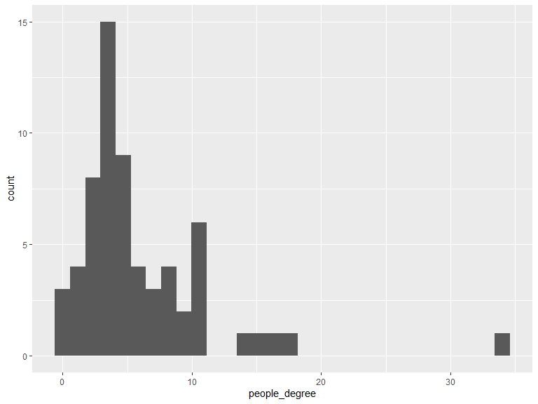

kable(t(as.matrix(summary(ess.tab.alex$people_degree))), caption = "people_degree") %>% kable_styling(bootstrap_options = "striped", full_width = T, position = "left")

people_degree

Min.	1st Qu.	Median	Mean	3rd Qu.	Max.
0	3	5	5.873016	8	34

3.10.6.2 Simmelian Brokerage (simmelian)

ggplot(ess.tab.alex) +
  geom_histogram(aes(x = simmelian))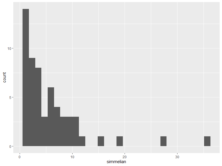

kable(t(as.matrix(summary(ess.tab.alex$simmelian))), caption = "simmelian") %>% kable_styling(bootstrap_options = "striped", full_width = T, position = "left")

simmelian

Min.	1st Qu.	Median	Mean	3rd Qu.	Max.	NA’s
1	2.020833	3.6	5.831426	7.623684	35.51515	5

3.10.6.3 Number of people with whom the participant like to socialize (socialize_size)

ggplot(ess.tab.alex) +
  geom_histogram(aes(x = socialize_size))

kable(t(as.matrix(summary(ess.tab.alex$socialize_size))), caption = "socialize_size") %>% kable_styling(bootstrap_options = "striped", full_width = T, position = "left")

socialize_size

Min.	1st Qu.	Median	Mean	3rd Qu.	Max.
0	2	3	4.142857	5	20

3.10.6.4 Weekly face-to-face interactions among people with whom the participant like to socialize (socialize_meet)

ggplot(filter(ess.tab.alex, socialize_meet < 100)) +
  geom_histogram(aes(x = socialize_meet)) +
  annotate(geom = "text", x = 75, y = 100, label = "X-axis: values over 100 not displayed", alpha = .5)

kable(t(as.matrix(summary(ess.tab.alex$socialize_meet))), caption = "socialize_meet") %>% kable_styling(bootstrap_options = "striped", full_width = T, position = "left")

socialize_meet

Min.	1st Qu.	Median	Mean	3rd Qu.	Max.
0	214	416	812.1111	728	18980

3.10.6.5 Weekly ICT interactions among people with whom the participant like to socialize (socialize_chat)

ggplot(filter(ess.tab.alex, socialize_chat < 100)) +
  geom_histogram(aes(x = socialize_chat)) +
  annotate(geom = "text", x = 55, y = 100, label = "X-axis: values over 100 not displayed", alpha = .5)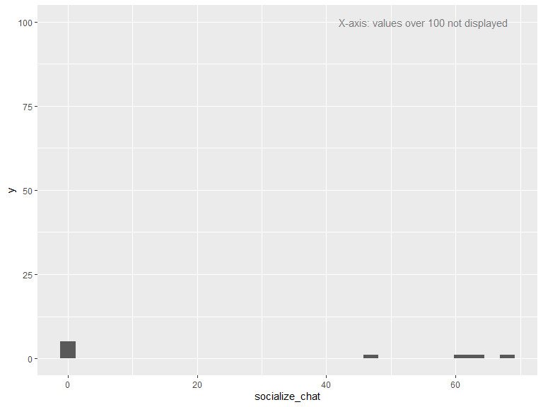

kable(t(as.matrix(summary(ess.tab.alex$socialize_chat))), caption = "socialize_chat") %>% kable_styling(bootstrap_options = "striped", full_width = T, position = "left")

socialize_chat

Min.	1st Qu.	Median	Mean	3rd Qu.	Max.
0	364	752	1289.19	1742	8840

3.10.6.6 Number of people with whom the participant discuss important matters (important_size)

ggplot(ess.tab.alex) +
  geom_histogram(aes(x = important_size))

kable(t(as.matrix(summary(ess.tab.alex$important_size))), caption = "important_size") %>% kable_styling(bootstrap_options = "striped", full_width = T, position = "left")

important_size

Min.	1st Qu.	Median	Mean	3rd Qu.	Max.
0	1	2	2.920635	4	19

3.10.6.7 Number of people in all groups (group_degree)

ggplot(filter(ess.tab.alex, group_degree < 100)) +
  geom_histogram(aes(x = group_degree)) +
  annotate(geom = "text", x = 20, y = 100, label = "X-axis: values over 100 not displayed", alpha = .5)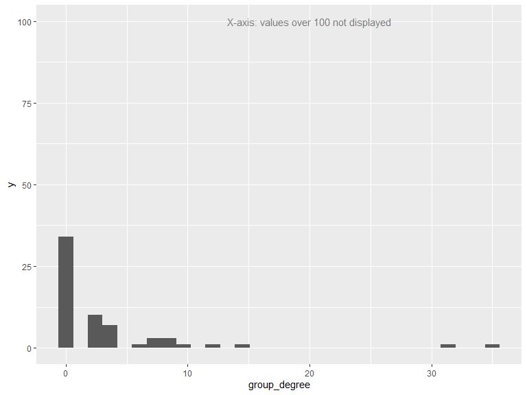

kable(t(as.matrix(summary(ess.tab.alex$group_degree))), caption = "group_degree") %>% kable_styling(bootstrap_options = "striped", full_width = T, position = "left")

group_degree

Min.	1st Qu.	Median	Mean	3rd Qu.	Max.
0	0	0	3.31746	4	35